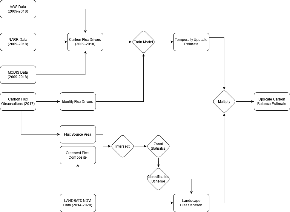
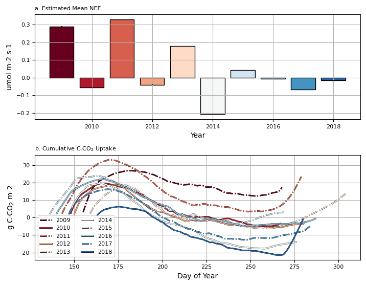
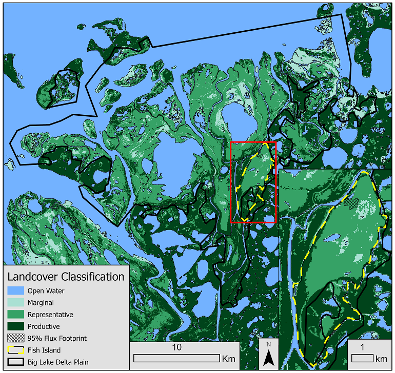
Footprint mapping, temporal upscaling. I’ll fill in more text here later, these figs are just grabbed from my thesis chapters. The gist of it - Measured NEE in one year. Have 10 years of climate data + Reanalysis data + satellite data. Combine these data sources & train a model to do a temporal upscale/sensitivity analysis to see how inter-annual climate variability impacts NEE. Then do a landscape classification with a greenest pixel NDVI image, intersecting with the flux footprint. Use that to find the representative areas to do a “back of the envelope” spatial upscaling.
Agriculture and Food, Ministry of. 1978. “Food Land Guidelines: A Policy Statement of the Government of Ontario on Planning for Agriculture.” Toronto: Government of Ontario.
Akaike, Hirotogu. 1973.
“Information Theory and an Extension of the Maximum Likelihood Principle.” In
In Proceedings of the 2nd International Symposium on Information Theory.
https://doi.org/10.1007/978-1-4612-1694-0_15.
Albers, Sam J. 2017.
“Tidyhydat: Extract and Tidy Canadian Hydrometric Data.” Journal of Open Source Software 2 (20): 511.
https://doi.org/10.21105/joss.00511.
American Society for Photogrammetry & Remote Sensing. 2019.
“LASER (LAS) FILE FORMAT EXCHANGE ACTIVITIES.” https://www.asprs.org/divisions-committees/lidar-division/laser-las-file-format-exchange-activities.
Anselin, Luc, and Anil Bera. 1998.
“Spatial Dependence in Linear Regression Models with an Introduction to Spatial Econometrics.” In
Handbook of Applied Economic Statistics, edited by A Ullah and D Giles, 237–89. New York: Marcel Dekker.
https://doi.org/10.1201/9781482269901-36.
Asa, Eric, Mohamed Saafi, Joseph Membah, and Arun Billa. 2012.
“Comparison of Linear and Nonlinear Kriging Methods for Characterization and Interpolation of Soil Data.” Journal of Computing in Civil Engineering 26 (1): 11–18.
https://doi.org/10.1061/(asce)cp.1943-5487.0000118.
Asner, Gregory P., Roberta E. Martin, David E. Knapp, Raul Tupayachi, Christopher Anderson, Loreli Carranza, Paola Martinez, Mona Houcheime, Felipe Sinca, and Parker Weiss. 2011.
“Spectroscopy of Canopy Chemicals in Humid Tropical Forests.” Remote Sensing of Environment 115 (12): 3587–98.
https://doi.org/10.1016/j.rse.2011.08.020.
Babak, Olena, and Clayton V. Deutsch. 2009.
“Statistical Approach to Inverse Distance Interpolation.” Stochastic Environmental Research and Risk Assessment 23 (5): 543–53.
https://doi.org/10.1007/s00477-008-0226-6.
Barber, C. Bradford, David P. Dobkin, and Hannu Huhdanpaa. 1996.
“The Quickhull Algorithm for Convex Hulls.” ACM Transactions on Mathematical Software 22 (4): 469–83.
https://doi.org/10.1145/235815.235821.
Bater, Christopher W. n.d. “Timelapse.”
Bater, Christopher W., Nicholas C. Coops, Michael A. Wulder, Thomas Hilker, Scott E. Nielsen, Greg Mcdermid, and Gordon B. Stenhouse. 2010.
“Using Digital Time-Lapse Cameras to Monitor Species-Specific Understorey and Overstorey Phenology in Support of Wildlife Habitat Assessment.” Environmental Monitoring and Assessment 180 (1-4): 1–13. https://doi.org/
http://dx.doi.org/10.1007/s10661-010-1768-x.
Biggs, Reinette, Alta de Vos, Rika Preiser, Hayley Clements, Kristine Maciejewski, and Maja Schlüter, eds. 2021.
The Routledge Handbook of Research Methods for Social-Ecological Systems. London: Routledge.
https://doi.org/10.4324/9781003021339.
Böhner, Jürgen, and Th Selige. 2006. “Spatial Prediction of Soil Attributes Using Terrain Analysis and Climate Regionalisation.”
Bouchard, Michelle A., and US Geological Survey. 2013.
“Example of the Landsat 8 Collection 2 Products U.S. Geological Survey.” https://www.usgs.gov/media/images/example-landsat-8-collection-2-products.
Burrough, Peter, and Rachael McDonnell. 1998.
“Principles of Geographical Information Systems by Peter A.” Oxford University Press 54 (2): 56–57.
https://doi.org/10.1111/j.1745-7939.1998.tb02089.x.
Canadian Space Agency, and NASA. 2019.
“Newfoundland – Earth as Seen by David Saint-Jacques.” https://www.asc-csa.gc.ca/eng/multimedia/search/Image/Watch/13330.
Carr, James R., and Nai hsien Mao. 1993.
“A General Form of Probability Kriging for Estimation of the Indicator and Uniform Transforms.” Mathematical Geology 25 (4): 425–38.
https://doi.org/10.1007/BF00894777.
———. n.d.b.
“Open Data Portal.” Accessed March 15, 2022.
https://opendata.vancouver.ca/.
City of Vancouver, Vancouver Board of Parks and Recreation. 2012.
“Street Trees.” https://opendata.vancouver.ca/explore/dataset/street-trees/.
Clark, Emily. 2016.
“Historical Trends of Ecosystem Services in Canada, 1911-2011.” PhD thesis, McGill University.
https://escholarship.mcgill.ca/concern/theses/pc289m86m?locale=en.
Clark, I, and W V Harper. 2007. Practical Geostatistics 2000. EcoSSe North America Llc, Ohio.
Cliff, J. K, A. D. and Ord. 1973. “Spatial Autocorrelation.” Progress in Human Geography 19: 245–49.
Coops, Nicholas C. n.d. “AMSPEC Radiometer.”
Coops, Nicholas C., Thomas Hilker, Michael A. Wulder, Benoît St-Onge, Glenn Newnham, Anders Siggins, and J. A. Trofymow. 2007.
“Estimating Canopy Structure of Douglas-Fir Forest Stands from Discrete-Return LiDAR.” Trees - Structure and Function 21 (3): 295–310.
https://doi.org/10.1007/s00468-006-0119-6.
Coulston, J W, and G A Reams. n.d. “The Effect of Blurred Plot Coordinates on Interpolating Forest Biomass : A Case Study 3041 Cornwallis Road 3041 Cornwallis Road” m.
Cressie, N. A. C. 1994.
“Statistics for Spatial Data, Revised Edition.” https://doi.org/10.2307/2533238.
Crist, Eric P., and Richard C. Cicone. 1984.
“A Physically-Based Transformation of Thematic Mapper Data—The TM Tasseled Cap.” IEEE Transactions on Geoscience and Remote Sensing GE-22 (3): 256–63.
https://doi.org/10.1109/TGRS.1984.350619.
Curran, Paul J. 1989.
“Remote Sensing of Foliar Chemistry.” Remote Sensing of Environment 30 (3): 271–78.
https://doi.org/10.1016/0034-4257(89)90069-2.
Dalponte, Michele, and David A. Coomes. 2016.
“Tree-Centric Mapping of Forest Carbon Density from Airborne Laser Scanning and Hyperspectral Data.” Methods in Ecology and Evolution 7 (10): 1236–45.
https://doi.org/10.1111/2041-210X.12575.
Daya, Ali Akbar, and Hadi Bejari. 2015.
“A Comparative Study Between Simple Kriging and Ordinary Kriging for Estimating and Modeling the Cu Concentration in Chehlkureh Deposit, SE Iran.” Arabian Journal of Geosciences 8 (8): 6003–20.
https://doi.org/10.1007/s12517-014-1618-1.
Deel, Lindsay N., Brenden E. McNeil, Philip G. Curtis, Shawn P. Serbin, Aditya Singh, Keith N. Eshleman, and Philip A. Townsend. 2012.
“Relationship of a Landsat Cumulative Disturbance Index to Canopy Nitrogen and Forest Structure.” Remote Sensing of Environment 118: 40–49.
https://doi.org/10.1016/j.rse.2011.10.026.
Delaunay, B. N. 1934. “Sur La Sphere Vide.” In Izvestia Akademia Nauk SSSR, VII Seria, Otdelenie Matematicheskii i Estestvennyka Nauk, 793–800. 7.
Deutsch, C, and A Journel. 1993. “GSLIB: Geostatistical Software Library and User’s Guide.” In.
DiBiase, David. 2014.
“Census Data and Thematic Maps.” In
Nature of Geographic Information.
https://opentextbc.ca/natureofgeographicinformation/chapter/1-overview-2/.
Dominion Bureau of Statistics. 1944. “Volume II: Population by Local Subdivisions.” Ottawa.
Earth Resources Observation and Science Center. 2018.
“USGS EROS Archive - Digital Elevation - Shuttle Radar Topography Mission (SRTM) 1 Arc-Second Global.” https://www.usgs.gov/centers/eros/science/usgs-eros-archive-digital-elevation-shuttle-radar-topography-mission-srtm-1.
Eash, David A., Kimberlee K. Barnes, Padraic S. O’Shea, and Brian K. Gelder. 2018.
“Stream-Channel and Watershed Delineations and Basin-Characteristic Measurements Using Lidar Elevation Data for Small Drainage Basins Within the Des Moines Lobe Landform Region in Iowa.” U.S. Geological Survey Scientific Investigations Report 2017–5108. https://doi.org/
https://doi.org/10.3133/sir20175108.
Engelsen, Ben den. 2020.
“Photo by Ben Den Engelsen on Unsplash.” https://unsplash.com/photos/UFwW97AP0LI.
Federation of Rocky Mountain States. Information Systems Technical Laboratory., U.S. Fish and Wildlife Service. Office of Biological Services., Western Energy and Land Use Team. 1977. “Comparison of Selected Operational Capabilities of Fifty-Four Geographic Information Systems.” FWS/OBS-77/54. Fort Collins, Colorado: Dept. of the Interior, Fish; Wildlife Service, Office of Biological Services, Western Energy; Land Use Team.
Finlayson, Graham D., and Steven D. Hordley. 2001.
“Color Constancy at a Pixel.” JOSA A 18 (2): 253–64.
https://doi.org/10.1364/JOSAA.18.000253.
Fisher, T, and C MacDonald. 1979.
“An Overview of the Canada Geographic Information System (CGIS).” In
Proceedings of the International Symposium on Cartography and Computing: Applications in Health and Environment, 1:610–15. Reston, Virginia.
https://cartogis.org/docs/proceedings/archive/auto-carto-4-vol-1/index3.html.
Forest Practices Branch, Ministry of Forests and Range. 2005.
“Silviculture Information Submission Guide.” https://www.for.gov.bc.ca/hfp/publications/00026/fs708-14-appendix_d.htm#ad_02.
Gallant, John C, and Trevor I Dowling. 2003. “A Multiresolution Index of Valley Bottom Flatness for Mapping Depositional Areas.” Water Resources Research 39 (12).
Geary, R . C . 1954.
“The Contiguity Ratio and Statistical Mapping.” The Incorporated Statistician 5 (3): 115–27.
https://www.jstor.org/stable/2986645.
Getis, Arthur, and Jared Aldstadt. 2010.
“Constructing the Spatial Weights Matrix Using a Local Statistic.” Advances in Spatial Science 61 (2): 147–63.
https://doi.org/10.1007/978-3-642-01976-0_11.
Getis, Arthur, Jesus Mur, Bernard Fingleton, and Maria Plotnikova. 2004. “Spatial Econometrics and Spatial Statistics Spatial Econometrics and Spatial Statistics Arthur Getis , Jesús Mur Lacambra and Henry G . Zoller,” no. May 2014.
Goodbody, Tristan R H, Nicholas C Coops, Joan E Luther, Piotr Tompalski, Christopher Mulverhill, Catherine Frizzle, Richard Fournier, Shane Furze, and Sam Herniman. 2021. “Airborne Laser Scanning for Quantifying Criteria and Indicators of Sustainable Forest Management in Canada” 985 (July): 972–85.
Goovaerts, Pierre. 2008.
“Kriging and Semivariogram Deconvolution in the Presence of Irregular Geographical Units.” Mathematical Geology 40 (1): 101–28.
https://www.ncbi.nlm.nih.gov/pmc/articles/PMC3624763/pdf/nihms412728.pdf.
Graham, R. 1972.
“An Efficient Algorithm for Determining the Convex Hull of a Finite Planar Set.” Information Processing Letters 1 (4): 132–33.
https://doi.org/10.1016/0020-0190(72)90045-2.
graph-tool. n.d.
“Centrality Measures.” Accessed March 15, 2022.
https://graph-tool.skewed.de/static/doc/centrality.html.
Gray, Walter. 1962. “Resources for Tomorrow.” The Globe and Mail, January, 7.
Greenlee, David D. 1987. “Raster and Vector Processing for Scanned Linework.” Photogrammetric Engineering and Remote Sensing 53 (10): 1383–87.
Hansen, M. C., P. V. Potapov, R. Moore, M. Hancher, S. A. Turubanova, A. Tyukavina, D. Thau, et al. 2013.
“High-Resolution Global Maps of 21st-Century Forest Cover Change.” Science 342 (6160): 850–53.
https://doi.org/10.1126/science.1244693.
Harker, K. J., L. Arnold, Ira J. Sutherland, and Sarah E. Gergel. 2021. “Perspectives from Landscape Ecology Can Improve Environmental Impact Assessment.” FACETS 6 (1): 358–78.
Hermosilla, Txomin, Michael A. Wulder, Joanne C. White, Nicholas C. Coops, and Geordie W. Hobart. 2018.
“Disturbance-Informed Annual Land Cover Classification Maps of Canada’s Forested Ecosystems for a 29-Year Landsat Time Series.” Canadian Journal of Remote Sensing 44 (1): 67–87.
https://doi.org/10.1080/07038992.2018.1437719.
Hesselbarth, M. H. K., M. Sciaini, K. A. With, K. Wiegand, and J. Nowosad. 2019.
“Landscapemetrics: An Open‐source R Tool to Calculate Landscape Metrics.” https://r-spatialecology.github.io/landscapemetrics/.
Hillier, Bill, Alan Penn, Julienne Hanson, T Grajewski, and J Xu. 1993.
“Natural Movement: Or, Configuration and Attraction in Urban Pedestrian Movement.” Environment and Planning B: Planning and Design 20 (1): 29–66.
https://doi.org/10.1068/b200029.
Howell, Carrie R., Wei Su, Ariann F. Nassel, April A. Agne, and Andrea L. Cherrington. 2020.
“Area Based Stratified Random Sampling Using Geospatial Technology in a Community-Based Survey.” BMC Public Health 20 (1): 1–9.
https://doi.org/10.1186/s12889-020-09793-0.
Huang, Chang, Ba Duy Nguyen, Shiqiang Zhang, Senmao Cao, and Wolfgang Wagner. 2017. “A Comparison of Terrain Indices Toward Their Ability in Assisting Surface Water Mapping from Sentinel-1 Data.” ISPRS International Journal of Geo-Information 6 (5): 140.
Hyyppä, Juha, and Mikko Inkinen. 1999. “Detecting and Estimating Attributes for Single Trees Using Laser Scanner.” The Photogrammetric Journal of Finland 16 (2): 27–42.
Iceton, Glenn. 2019.
“"Many Families of Unseen Indians": Trapline Registration and Understandings of Aboriginal Title in the BC-Yukon Borderlands.” BC Studies, no. 201: 67–91, 175.
https://www.proquest.com/docview/2265666649/abstract/665EA1CCEFE34A59PQ/1.
Inamdar, Deep, Margaret Kalacska, George Leblanc, and J Pablo Arroyo Mora. 2020.
“Characterizing and Mitigating Sensor Generated Spatial Correlations in Airborne Hyperspectral Imaging Data.” https://doi.org/10.3390/rs12040641.
Isaaks, Edward, and R.Mohan Srivastava. 1989.
An Introduction to Applied Geostatistics. 1st ed. Vol. 17. 3. New York: Oxford University Press, New York. https://doi.org/
https://doi.org/10.1016/0098-3004(91)90055-I.
Jaboyedoff, Michel, Thierry Oppikofer, Antonio Abellán, Marc Henri Derron, Alex Loye, Richard Metzger, and Andrea Pedrazzini. 2012.
“Use of LIDAR in Landslide Investigations: A Review.” Natural Hazards 61 (1): 5–28.
https://doi.org/10.1007/s11069-010-9634-2.
Jackson, Michelle, Sarah Gergel, and Kathy Martin. 2015.
“Citizen Science and Field Survey Observations Provide Comparable Results for Mapping Vancouver Island White-Tailed Ptarmigan (Lagopus Leucura Saxatilis) Distributions.” Biological Conservation 181 (6).
https://doi.org/10.1016/j.biocon.2014.11.010.
Jacquez, Geoffrey M. 1999.
“Spatial Statistics When Locations Are Uncertain.” Geographic Information Sciences 5 (2): 77–87.
https://doi.org/10.1080/10824009909480517.
Jakubowski, Marek K., Wenkai Li, Qinghua Guo, and Maggi Kelly. 2013.
“Delineating Individual Trees from Lidar Data: A Comparison of Vector- and Raster-Based Segmentation Approaches.” Remote Sensing 5 (9): 4163–86.
https://doi.org/10.3390/rs5094163.
Jarvis, R. A. 1973.
“On the Identification of the Convex Hull of a Finite Set of Points in the Plane.” Information Processing Letters 2 (1): 18–21.
https://doi.org/10.1016/0020-0190(73)90020-3.
Journel, A. G. 1983.
“Nonparametric Estimation of Spatial Distributions.” Journal of the International Association for Mathematical Geology 15 (3): 445–68.
https://doi.org/10.1007/BF01031292.
Kassen, Maxat. 2013.
“A Promising Phenomenon of Open Data: A Case Study of the Chicago Open Data Project.” Government Information Quarterly 30 (4): 508–13.
https://doi.org/10.1016/j.giq.2013.05.012.
Key, C. H., and N. C. Benson. 2006.
“Landscape Assessment: Ground Measure of Severity, the Composite Burn Index; and Remote Sensing of Severity, the Normalized Burn Ratio.” RMRS-GTR-164-CD: LA 1-51. Ogden, UT: USDA Forest Service, Rocky Mountain Research Station.
https://pubs.er.usgs.gov/publication/2002085.
Krige, D. G. 1951. “A Statistical Approach to Some Basic Mine Valuation Problems on the Witwatersrand.” Journal of Southern African Institute of Mining and Metallurgy 52 (6): 119–39.
La Bella, Laura. 2009. Not Enough to Drink: Pollution, Drought, and Tainted Water Supplies. New York: The Rosen Publishing Group.
Lee, Kathryn A., Jonathan R. Lee, and Patrick Bell. 2020.
“A Review of Citizen Science Within the Earth Sciences: Potential Benefits and Obstacles.” Proceedings of the Geologists’ Association 131 (6): 605–17.
https://doi.org/10.1016/j.pgeola.2020.07.010.
Leggett, Gordon. 2014.
“Google Maps Car and Camera Used for Collecting Street View Data in Steveston, BC Canada.” https://commons.wikimedia.org/wiki/File:2014-04-29_Google_Maps_Streetview_car.jpg.
Library and Archives Canada. 1917.
“Athabasca Glacier from Below Wilcox Peak.” https://central.bac-lac.gc.ca/.redirect?app=fonandcol&id=4939507&lang=eng.
Lim, Kevin, Paul Treitz, Michael Wulder, Benoît St-Ongé, and Martin Flood. 2003.
“LiDAR Remote Sensing of Forest Structure.” Progress in Physical Geography 27 (1): 88–106.
https://doi.org/10.1191/0309133303pp360ra.
Little, Patrick J., John S. Richardson, and Younes Alila. 2013.
“Channel and Landscape Dynamics in the Alluvial Forest Mosaic of the Carmanah River Valley, British Columbia, Canada.” Geomorphology 202 (November): 86–100.
https://doi.org/10.1016/j.geomorph.2013.04.006.
López García, M. J., and V. Caselles. 1991.
“Mapping Burns and Natural Reforestation Using Thematic Mapper Data.” Geocarto International 6 (1): 31–37.
https://doi.org/10.1080/10106049109354290.
Maguire, Kyle. n.d.a. “Mt. Assiniboine, Day.”
———. n.d.b. “Mt. Assiniboine, Sunset.”
Makarau, Aliaksei, Rudolf Richter, Rupert Müller, and Peter Reinartz. 2014.
“Haze Detection and Removal in Remotely Sensed Multispectral Imagery.” IEEE Transactions on Geoscience and Remote Sensing 52 (9): 5895–905.
https://doi.org/10.1109/TGRS.2013.2293662.
Manning, E. W., and J. D. McCuaig. 1977. “An Overview of the Significance of Urban Centres to Canada’s Quality Agricultural Land.” Report Number 11. Ottawa: Fisheries; Environment Canada Lands Directorate.
Marks, Danny, Jeff Dozier, and James Frew. 1984. “Automated Basin Delineation from Digital Elevation Data.” Geo-Processing 2: 299–311.
Martino, Nicholas. 2020.
“Spatial Network Analysis.” https://ubc-library-rc.github.io/qgis-walkability/.
Matheron, G. 1962.
Traité de Géostatistique Appliquée. Memoires, v. 1. Éditions Technip.
https://books.google.ca/books?id=88YKAQAAMAAJ.
Matheron, G. 1973.
“Intrinsic Random Functions and Their Applications.” Advances in Applied Probability 5 (3): 439–68.
https://doi.org/10.1017/S0001867800039379.
Mattivi, Pietro, Francesca Franci, Alessandro Lambertini, and Gabriele Bitelli. 2019. “TWI Computation: A Comparison of Different Open Source GISs.” Open Geospatial Data, Software and Standards 4 (1): 1–12.
MAXAR. n.d.
“Precision3D Data Suite.” Accessed March 14, 2022.
https://www.maxar.com/products/precision3d-data-suite.
McClenachan, Loren, Andrew B. Cooper, Matthew G. McKenzie, and Joshua A. Drew. 2015.
“The Importance of Surprising Results and Best Practices in Historical Ecology.” BioScience 65 (9): 932–39.
https://doi.org/10.1093/biosci/biv100.
McCrorie, James. 1969. “ARDA: An Experiment in Development Planning.” Special Study 2. Ottawa: Canadian Council on Rural Development.
McCune, Bruce, and Dylan Keon. 2002.
“Equations for Potential Annual Direct Incident Radiation and Heat Load.” Journal of Vegetation Science 13 (August): 603–6.
https://doi.org/10.1111/j.1654-1103.2002.tb02087.x.
McRoberts, R. E., E. O. Tomppo, and R. L. Czaplewski. 2014.
“Sampling Designs for National Forest Assessments: Knowledge Reference for National Forest Assessments.” Food and Agricultural Organisation of the UN (FAO), 23–40.
http://www.fao.org/%0Aforestry/44859-02cf95ef26dfdcb86c6be2720f8b938a8.pdf. Rome. FAO.
Meng, Qingmin, Chris J. Cieszewski, Mike R. Strub, and Bruce E. Borders. 2009.
“Spatial Regression Modeling of Tree Height-Diameter Relationships.” Canadian Journal of Forest Research 39 (12): 2283–93.
https://doi.org/10.1139/X09-136.
Monniaux, David, cmglee, and jimhtatshawdotca. 2005.
“Illustration of the Method Eratosthenes Used to Calculate the Circumference of the Earth.” https://commons.wikimedia.org/wiki/File:Eratosthenes_measure_of_Earth_circumference.svg.
Moran, P. 1950. “Notes on Continuous Stochastic Phenomenon.” Biometrika 37 (1): 17–23.
Morgan, J. L., S. Gergel, Collin Ankerson, S. Tomscha, and Ira J. Sutherland. 2017.
“Historical Aerial Photography for Landscape Analysis.” In
Learning Landscape Ecology, 21–40. Springer, New York, NY.
https://doi.org/10.1007/978-1-4939-6374-4_2.
Morsy, Salem, Ahmed Shaker, and Ahmed El-Rabbany. 2017.
“Multispectral Lidar Data for Land Cover Classification of Urban Areas.” Sensors (Switzerland) 17 (5).
https://doi.org/10.3390/s17050958.
Mountain Legacy Project. 2011.
“Modern Athabasca Glacier.” http://mountainlegacy.ca/.
Nadar. 1868.
“The Arc de Triomphe and the Grand Boulevards, Paris, from a Balloon.” https://commons.wikimedia.org/wiki/File:Nadar_triomphe_1868.jpg.
Næsset, Erik. 2002.
“Predicting Forest Stand Characteristics with Airborne Scanning Laser Using a Practical Two-Stage Procedure and Field Data.” Remote Sensing of Environment 80 (1): 88–99.
https://doi.org/10.1016/S0034-4257(01)00290-5.
NASA. n.d.a.
“Atmospheric Transmission.” Accessed March 16, 2022.
https://landsat.gsfc.nasa.gov/satellites/landsat-8/.
———. n.d.b.
“GOES-1 Satellite.” keeptrack.space.
NASA, and Tom Neumann. 2021.
“IceSat-2; Ice, Cloud, AND LAND ELEVATION SA℡LITE-2.” https://icesat-2.gsfc.nasa.gov/.
NASA, and University of Maryland. 2021.
“GEDI Ecosystem LiDAR.” https://gedi.umd.edu/.
Native Land. n.d.
“Native Land Digital.” Accessed March 29, 2022.
https://native-land.ca/.
Natural Resources Canada. 2015.
“Canadian Digital Elevation Model, 1945-2011.” https://open.canada.ca/data/en/dataset/7f245e4d-76c2-4caa-951a-45d1d2051333.
———. n.d.a.
“Earth Observation Data Management System.” Accessed March 29, 2022.
https://www.eodms-sgdot.nrcan-rncan.gc.ca/index-en.html.
———. n.d.b.
“Natural Resources Canada.” Accessed March 29, 2022.
https://www.nrcan.gc.ca/home.
Natural Resources Canada, Canadian Forest Service. 2013.
“Douglas-Fir and Western Hemlock.” Trees, Insects and Diseases of Canada’s Forests.
https://tidcf.nrcan.gc.ca/en/trees/factsheet/119.
Nelson, Ross. 2013.
“How Did We Get Here? An Early History of Forestry Lidar.” Canadian Journal of Remote Sensing 39 (SUPPL.1).
https://doi.org/10.5589/m13-011.
NEON Education. 2014.
“A Key Component of a Lidar System Is a GPS.” https://www.flickr.com/photos/128087132@N06/15408803390.
NRCAN. 2021.
“Canadian Digital Elevation Model Earth Engine Data Catalog.” Canadian Digital Elevation Model.
https://developers.google.com/earth-engine/datasets/catalog/NRCan_CDEM.
Okabe, Atsuyuki, Barry Boots, and Kokichi Sugihara. 1994.
“Nearest Neighbourhood Operations with Generalized Voronoi Diagrams: A Review.” International Journal of Geographical Information Systems 8 (1): 43–71.
https://doi.org/10.1080/02693799408901986.
OpenStreetMap. n.d. Accessed March 14, 2022.
https://www.openstreetmap.org/copyright.
Oregon Department of Transportation. 2016.
“3D Mobile Mapping Unit.” https://www.flickr.com/photos/oregondot/24784201084/in/photostream/.
Oxford Languages. n.d.
“Phenomena.” Accessed March 21, 2022.
https://languages.oup.com/google-dictionary-en/.
Parker, J. Anthony, Robert V. Kenyon, and Donald E. Troxel. 1983.
“Comparison of Interpolating Methods for Image Resampling.” IEEE Transactions on Medical Imaging 2 (1): 31–39.
https://doi.org/10.1109/TMI.1983.4307610.
“Parliamentary Debates (Hansard).” 2001.
Pickell, Paul, Nicholas Coops, Colin Ferster, Christopher Bater, Karen Blouin, Mike Flannigan, and Jinkai Zhang. 2017.
“An Early Warning System to Forecast the Close of the Spring Burning Window from Satellite-Observed Greenness.” Scientific Reports 7 (1).
https://doi.org/10.1038/s41598-017-14730-0.
Potapov, Peter, Xinyuan Li, Andres Hernandez-Serna, Alexandra Tyukavina, Matthew C. Hansen, Anil Kommareddy, Amy Pickens, et al. 2021.
“Mapping Global Forest Canopy Height Through Integration of GEDI and Landsat Data.” Remote Sensing of Environment 253 (February).
https://doi.org/10.1016/j.rse.2020.112165.
Qin, C., A.‐X. Zhu, T. Pei, B. Li, C. Zhou, and L. Yang. 2007.
“An Adaptive Approach to Selecting a Flow‐partition Exponent for a Multiple‐flow‐direction Algorithm.” International Journal of Geographical Information Science 21 (4): 443–58.
https://doi.org/10.1080/13658810601073240.
Quartl. 2012.
“English: Illustration of the Cartesian Product A x B of Two Sets A={x,y,z} and B={1,2,3}.” https://commons.wikimedia.org/wiki/File:Cartesian_Product_qtl1.svg.
Quey, Romain. n.d.
“Neper.” Accessed March 29, 2022.
https://github.com/rquey/neper.
Ramsey, Paul. 2012.
“23. Linear Referencing — Introduction to PostGIS.” http://postgis.net/workshops/postgis-intro/linear_referencing.html.
Raney, R. K., A. P. Luscombe, E. J. Langham, and S. Ahmed. 1991.
“RADARSAT (SAR Imaging).” Proceedings of the IEEE 79 (6): 839–49.
https://doi.org/10.1109/5.90162.
Regional Economic Expansion, Department of. 1965. “The Canada Land Inventory: Objectives, Scope, and Organization.” Report 1. Ottawa: Queen’s Printer for Canada.
Rossi, Richard E., David J. Mulla, André G. Journel, and Eldon H. Franz. 1992.
“Geostatistical Tools for Modeling and Interpreting Ecological Spatial Dependence.” Ecological Monographs 62 (2): 277–314.
https://doi.org/10.2307/2937096.
Rouse, J. W., R. H. Haas, J. A. Schell, and D. W. Deering. 1974.
“Monitoring Vegetation Systems in the Great Plains with ERTS.” In
NASA. Goddard Space Flight Center 3d ERTS-1 Symp. Vol. 1.
https://ntrs.nasa.gov/citations/19740022614.
Roussel, Jean Romain, David Auty, Nicholas C. Coops, Piotr Tompalski, Tristan R. H. Goodbody, Andrew Sánchez Meador, Jean François Bourdon, Florian de Boissieu, and Alexis Achim. 2020.
“lidR: An R Package for Analysis of Airborne Laser Scanning (ALS) Data.” Remote Sensing of Environment 251 (August): 112061.
https://doi.org/10.1016/j.rse.2020.112061.
Roussel, Jean-Romain, Tristan R. H. Goodbody, and Piotr Tompalski. 2021.
“lidR Book.” https://r-lidar.github.io/lidRbook/.
Shepard, D. 1968. “Two- Dimensional Interpolation Function for Irregularly- Spaced Data.” Proc 23rd Nat Conf, 517–24.
Shreve, Ronald L. 1966. “Statistical Law of Stream Numbers.” The Journal of Geology 74 (1): 17–37.
Skeeter, June, Andreas Christen, and Greg H. R. Henry. 2022.
“Controls on Carbon Dioxide and Methane Fluxes from a Low-Center Polygonal Peatland in the Mackenzie River Delta.” Arctic Science, February.
https://doi.org/10.1139/AS-2021-0034.
Snyder, John Parr. 1987. Map Projections–A Working Manual. Vol. 1395. US Government Printing Office.
Special Committee on Land Use in Canada. 1963. “Consolidation of the Proceedings and Considerations of the Committee from Its Inception on January 30, 1957 to the End of the First Session 25th Parliament, February 6th, 1963 on Land Use in Canada.”
Statistics Canada. n.d.
“Statistics Canada.” Accessed March 29, 2022.
https://www.statcan.gc.ca/en/start.
Statistics Canada, Government of Canada. 2019.
“Canadian Index of Multiple Deprivation: Dataset.” https://www150.statcan.gc.ca/n1/pub/45-20-0001/452000012019001-eng.htm.
Steel, R G, and J Torrie. 1980. “Principles and Procedures of Statistics: A Biometrical Approach (2nd Ed).” In.
Stein, Ayal, Eran Geva, and Jihad El-Sana. 2012.
“CudaHull: Fast Parallel 3D Convex Hull on the GPU.” Computers & Graphics, Applications of
Geometry Processing, 36 (4): 265–71.
https://doi.org/10.1016/j.cag.2012.02.012.
Strahler, Arthur N. 1957. “Quantitative Analysis of Watershed Geomorphology.” Eos, Transactions American Geophysical Union 38 (6): 913–20.
Suryowati, K., R. D. Bekti, and A. Faradila. 2018.
“A Comparison of Weights Matrices on Computation of Dengue Spatial Autocorrelation.” IOP Conference Series: Materials Science and Engineering 335 (1).
https://doi.org/10.1088/1757-899X/335/1/012052.
Swatantran, Anu, Hao Tang, Terence Barrett, Phil Decola, and Ralph Dubayah. 2016.
“Rapid, High-Resolution Forest Structure and Terrain Mapping over Large Areas Using Single Photon Lidar.” Scientific Reports 6 (June): 1–12.
https://doi.org/10.1038/srep28277.
Systems Innovation. 2015a.
“Graph Theory Overview.” https://youtu.be/82zlRaRUsaY.
———. 2015b.
“Network Diffusion & Contagion.” https://youtu.be/bTXUJQhEqL0.
Tarboton, David G. 1997.
“A New Method for the Determination of Flow Directions and Upslope Areas in Grid Digital Elevation Models.” Water Resources Research 33 (2): 309–19.
https://doi.org/10.1029/96WR03137.
Tashakkori, Abbas, and Charles Teddlie. 2010.
“SAGE Handbook of Mixed Methods in Social & Behavioral Research.” https://doi.org/10.4135/9781506335193.
Teddlie, Charles, and Fen Yu. 2007.
“Mixed Methods Sampling: A Typology With Examples.” Journal of Mixed Methods Research 1 (1): 77–100.
https://doi.org/10.1177/2345678906292430.
The Center for International Forestry Research (CIFOR). 2014.
“LiDAR Machine.” https://www.flickr.com/photos/cifor/36019786455/.
The Good Doctor Fry. 2011.
“Diagram of Scattering of Sunlight to Make a Yellow/Red Appearing Sun and Blue Sky.” https://commons.wikimedia.org/wiki/File:Rayleigh_mie_fry3a.jpg.
The Senate of Canada. 1957. “Minutes of the Proceedings of the Senate of Canada.”
Thompson, S K. 2012.
Sampling.
CourseSmart. Wiley.
https://books.google.ca/books?id=-sFtXLIdDiIC.
Thompson, Shanley D., Trisalyn A. Nelson, Joanne C. White, and Michael A. Wulder. 2015.
“Mapping Dominant Tree Species over Large Forested Areas Using Landsat Best-Available-Pixel Image Composites.” Canadian Journal of Remote Sensing 41 (3): 203–18.
https://doi.org/10.1080/07038992.2015.1065708.
Titus, Jency, and Sebastian Geroge. 2013.
“A Comparison Study On Different Interpolation Methods Based On Satellite Images.” International Journal of Engineering Research & Technology 2 (6): 82–85.
www.ijert.org.
Tomlinson, Matthew J., Sarah E. Gergel, Timothy J. Beechie, and Michelle M. McClure. 2011.
“Long-Term Changes in River—Floodplain Dynamics: Implications for Salmonid Habitat in the Interior Columbia Basin, USA.” Ecological Applications 21 (5): 1643–58.
https://www.jstor.org/stable/23023107.
Tomlinson, Roger. 1967. An Introduction to the Geo-Information System of the Canada Land Inventory. Ottawa: Department of Forestry; Rural Development.
———. 1974. “The Application of Electronic Computing Methods and Techniques to the Storage, Compilation, and Assessment of Mapped Data.” Dissertation, London: University of London.
Tompalski, Piotr, Joanne C. White, Nicholas C. Coops, and Michael A. Wulder. 2019.
“Demonstrating the Transferability of Forest Inventory Attribute Models Derived Using Airborne Laser Scanning Data.” Remote Sensing of Environment 227 (September 2018): 110–24.
https://doi.org/10.1016/j.rse.2019.04.006.
Tomscha, Stephanie A., Ira J. Sutherland, Delphine Renard, Sarah E. Gergel, JEANINE M. Rhemtulla, Elena M. Bennett, Lori D. Daniels, Ian M. S. Eddy, and Emily E. Clark. 2016.
“A Guide to Historical Data Sets for Reconstructing Ecosystem Service Change over Time.” BioScience 66 (9): 747–62.
https://www.jstor.org/stable/90007657.
Tziachris, Panagiotis, Eirini Metaxa, Frantzis Papadopoulos, and Maria Papadopoulou. 2017.
“Spatial Modelling and Prediction Assessment of Soil Iron Using Kriging Interpolation with pH as Auxiliary Information.” ISPRS International Journal of Geo-Information 6 (9).
https://doi.org/10.3390/ijgi6090283.
UF Geomatics - Fort Lauderdale. 2016a.
“LiDAR Remote Sensing Part 1: Principles.” EcoLearnIT.
https://youtu.be/T5hFrS57LGo.
———. 2016b.
“LiDAR Remote Sensing Part 2: Systems & Data Collection.” EcoLearnIT.
https://youtu.be/jS0lI-ZMSSo.
———. 2016c.
“LiDAR Remote Sensing Part 3: Data Analysis.” EcoLearnIT.
https://youtu.be/wpW1cx7WMXQ.
University, Kent State. 1968. “The Cuyahoga River Watershed.” In Proceedings of a Symposium Commemorating the Dedication of Cunningham Hall. Cleveland: Kent State University.
USGS. n.d.
“Copyrights and Credits U.S. Geological Survey.” Accessed March 22, 2022.
https://www.usgs.gov/information-policies-and-instructions/copyrights-and-credits.
Ustin, Susan L., and Michael E. Schaepman. 2009.
“Imaging Spectroscopy Special Issue.” Remote Sensing of Environment 113 (SUPPL. 1): S1.
https://doi.org/10.1016/j.rse.2008.09.018.
Wackernagel, Hans. 2002.
Multivariate Geostatistics: An Introduction with Applications. 3rd ed. Springer.
https://doi.org/10.1007/978-3-662-05294-5.
Wang, Ran, John A. Gamon, Jeannine Cavender-Bares, Philip A. Townsend, and Arthur I. Zygielbaum. 2018.
“The Spatial Sensitivity of the Spectral Diversity-Biodiversity Relationship: An Experimental Test in a Prairie Grassland.” Ecological Applications 28 (2): 541–56.
https://doi.org/10.1002/eap.1669.
Wegmann, Martin. 2011.
“Hemispherical Photo in the Bavarian Forest.” https://commons.wikimedia.org/wiki/File:Hemispherical_photo1.jpg.
White, Joanne C., Michael A. Wulder, Andrés Varhola, Mikko Vastaranta, Nicholas C. Coops, Bruce D Cook, Doug Pitt, and Murray Woods. 2013.
“A Best Practices Guide for Generating Forest Inventory Attributes from Airborne Laser Scanning Data Using an Area-Based Approach. Information Report FI-X-010.” Victoria, BC, Canada: Canadian Forest Service, Canadian Wood Fibre Centre, Pacific Forestry Centre.
https://doi.org/10.5558/tfc2013-132.
Wikimedia. 2021a. “Delaunay Triangulation.” Wikipedia, July.
———. 2021b. “PageRank.” Wikipedia, July.
Wilkes, Phil, Simon D. Jones, Lola Suarez, Andrew Haywood, William Woodgate, Mariela Soto-Berelov, Andrew Mellor, and Andrew K. Skidmore. 2015.
“Understanding the Effects of ALS Pulse Density for Metric Retrieval Across Diverse Forest Types.” Photogrammetric Engineering & Remote Sensing 81 (8): 625–35.
https://doi.org/10.14358/PERS.81.8.625.
Wolchover, Natalie. 2012.
“How Far Can the Human Eye See?” Livescience.com.
https://www.livescience.com/33895-human-eye.html.
Yamada, Ikuho. 2016.
“Thiessen Polygons.” International Encyclopedia of Geography: People, the Earth, Environment and Technology, 1–6.
https://doi.org/10.1002/9781118786352.wbieg0157.
Yates, S. R., A. W. Warrick, and D. E. Myers. 1986.
“Disjunctive Kriging: 2. Examples.” Water Resources Research 22 (5): 623–30.
https://doi.org/10.1029/WR022i005p00623.
Zurqani, Hamdi A., Christopher J. Post, Elena A. Mikhailova, Michael P. Cope, Jeffery S. Allen, and Blake A. Lytle. 2020.
“Evaluating the Integrity of Forested Riparian Buffers over a Large Area Using LiDAR Data and Google Earth Engine.” Scientific Reports 10 (1): 1–16.
https://doi.org/10.1038/s41598-020-69743-z.
Zwinkels, Joanne. 2020.
“Encyclopedia of Color Science and Technology.” Encyclopedia of Color Science and Technology, 1–8.
https://doi.org/10.1007/978-3-642-27851-8.
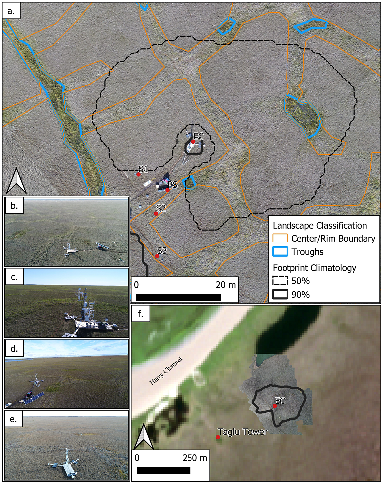
![The Eddy Covariance system at Fish Island [@skeeter_controls_2022].](images/16-ec-site.png)
![Maybe insert Web-map showing site instead. [@skeeter_controls_2022]](images/16-fig1.png)
![Precision versus accuracy [@davies_precision_2020].](images/16-accuracy-vs-precision.png)
![Accuracy and precision in chronostratigraphy [@davies_accuracy_2020].](images/16-accuracy-vs-precision2.png)