Chapter 7 Network Analysis
Written by Nicholas Martino and Paul Pickell
Networks are abstract structures commonly used to represent patterns of relationships among sets of various things (Ajorlou 2018). Such structures can be used to represent social connections, spatial patterns, ecological relationships, etc. In GIS, the elements that compose geospatial networks are geolocated – in other words: they have latitude and longitude values attached to them. Network analysis encompasses a series of techniques used to interpret information from those networks. This chapter introduces basic concepts for building, analyzing and applying spatial networks to real-world problems.
- Understand what networks are and to identify the elements that compose them
- Categorize different types of networks according to their topologies
- Create spatial networks and learn how to apply them in various applications
- Extract relevant information from spatial networks about the relationship between their elements, such as routes, distances and centralities
7.1 Introduction to Graph Theory
Graphs are the abstract language of networks (Systems Innovation 2015a). Graph theory is the area of mathematics that study graphs. By abstracting networks into graphs, one is able to measure different kinds of indicators that represents information about relationships that exist within a certain system. Why abstracting real-world elements into networks can be useful? Network analysis facilitates the study of data sets that demand information about their behaviour in terms of connectivity, flows, direction or paths. This is especially useful to understand the behaviour of complex adaptive systems such as societies, cities, ecosystems, etc. All graphs are composed of two parts: nodes and edges (or links).
7.2 Nodes
A node (or vertex) may represent any thing that can be connected with other things. For example, it can represent people in social networks, street intersections in road networks, or chemical compounds in molecular networks, among others.
7.3 Edges
Edges (or links), on the other hand, represent how vertices are interconnected to each other. So it may represent the vertices’ social connections, street segments, molecular bindings, etc. The graph below represents rapid and frequent transit lines in Metro Vancouver. Each node represents a transit line and the edges represents connections between those lines.
Figure 7.1: Graph representing connection between Metro Vancouver rapid and frequent transit lines. Interactive figure in the online format of the textbook.
![Rapid and frequent transit network in Metro Vancouver [@translink_2020_2020].](images/08-metro_vancouver_transit_network.png)
Figure 7.2: Rapid and frequent transit network in Metro Vancouver (TransLink 2020).
7.4 Connectivity and Order
There are two major types of connections within the graphs: directed and undirected. Connections are directed when they have a specific node of origin and destination.
7.5 Direct
Directed graphs are networks where the order of elements change relationships between them. We represent directed connections with an arrow. The network below represents relationships between characters of Les Miserables. For example, in the case of the transit network we could use a directed graph to represent the path one has to take in order to shift from one line to another.
Figure 7.3: Example of directed graph for social relationships. Interactive figure in the online format of the textbook.
7.6 Undirect
On the other hand, in an undirected graph, connections are represented as simple lines instead of arrows. The order of elements does not matter.
7.7 Network Topologies
Topology is the study of how network elements are arranged. The same elements arranged in different ways can change the network structure and dynamics. A very common example is the arrangement of computer networks.
![Abstract examples of network topologies [@wikibooks_communication_2018].](images/08-network_topologies.png)
Figure 7.4: Abstract examples of network topologies (Wikibooks 2018).
7.8 Physical vs. Logical Topology
In GIS we use networks to represent spatial structures of various kinds. While all networks can be represented in an abstract space - this is, without a defined position in the real-world - some network analysis might be more useful when we attach physical properties to them, such as latitude and longitude coordinates. We call logical topology the study of how network elements are arranged in this abstract space. On the other hand, physical topology refers to the arrangemet of networks in the physical space. We can then classify “types” of networks according to the way their nodes is arranged.
7.9 Non-Hierarchical Topologies
7.9.1 Lines
Lines are when nodes are arranged in series where every node has no more than two connections, except for the two end nodes. A rail transit line, for example, can be represented as a line network. The map below portrays the SkyTrain Millenium Line in Vancouver. Each node represents a stop and the lines the connections between those stops.
Figure 7.5: Rail transit line in Vancouver (City of Vancouver n.d.b). Licensed under the Open Government License - Vancouver.
7.9.2 Rings
Rings are similar to lines except that there are no end nodes. So each and every node has two connections and the “first” and “last” nodes are connected to each other forming a circle. The spatial structure of the Stanley park seawall trail in Vancouver resembles a ring. In this example, nodes stand for intersections and view spots and edges are the connections between these spots along the seawall.
Figure 7.6: Ring of the Stanley Park seawall (City of Vancouver n.d.b). Licensed under the Open Government License - Vancouver.
7.9.3 Meshes
In a mesh, every node is also connected to more than one node. However, in this case nodes can be connected to more than two nodes. Connections in a mesh are non-hierarchical. Contrary to rings and lines where there is only one possible route from one node to another, in a mesh there are multiple routes to access other nodes in the network. A common way to generate a mesh network is using Delaunay triangulation, where nodes are connected in order to form triangles and maximize the minimum angle of all triangles (Wikimedia 2021a). Mesh configurations are commonly used in decentralized structures such as the internet.
Figure 7.7: Tree canopy mesh (City of Vancouver n.d.b). Licensed under the Open Government License - Vancouver.
7.9.4 Fully Connected
As the name suggests, in fully connected networks every node is connected to every other node. The graph representing all possible origin-destination commutes among Metro Vancouver municipalities is a type of fully connected network.
Figure 7.8: Possible origin-destination commutes between municipalities within Metro Vancouver (City of Vancouver n.d.b). Licensed under the Open Government License - Vancouver.
7.10 Hierarchical Topologies
Different from non-hierarchical topologies, hierarchical configurations are structured around a central node or link. By looking into hierarchical topologies it becomes easier to understand the notion of depth. The more distant a node is from the central node or link, the more depth it has. Hover the mouse over the nodes in the following maps to check out their depth.
7.10.1 Stars
Stars are hierarchical structures where two or more nodes are directly connected to a central node. This concentric garden at the University of British Columbia can be represented according to a star topology.
Figure 7.9: Spatial structure of a concentric garden at UBC (City of Vancouver n.d.b). Licensed under the Open Government License - Vancouver.
7.10.2 Buses
Buses are structures where every path from one node to another passes through a central path or corridor. If we isolate a street segment from an urban street network, the connections between buildings and streets depict a bus topology.
Figure 7.10: Connections between houses and streets (City of Vancouver n.d.b). Licensed under the Open Government License - Vancouver.
7.10.3 Trees
In tree topologies, nodes are structured from a root node and arranged into edges that are similar to branches of a tree. This highly hierarchical structure create a sort of parent - child relationship amongst nodes. The spatial configuration of boat marinas are usually structures in tree-like topologies. By definition, all tree network structures will always have more than one terminal nodes (a node that only has one connection to the network).
Figure 7.11: Tree spatial structure of a boat marina (City of Vancouver n.d.b). Licensed under the Open Government License - Vancouver.
7.11 Spatial Network Analysis
Networks can then be arranged according to various different configurations. Aside from classifying networks into different types according to their topologies, some of the most useful features of spatial network analysis refers to how to extract information from these structures given certain parameters.
7.12 Network Tracing
The act of modelling spatial networks is called network tracing. When tracing a network it is important to bear in mind the direction with which information is added to the network, especially when this orientation information is important to further analyze flows and relationships within such structure. For example, when mapping hydrological networks to study its flows it might be useful to model the direction of streams coherently as this might be an important information to represent the dynamics of the network.
Figure 7.12: Graph representing Fraser River Flows (City of Vancouver n.d.b). Licensed under the Open Government License - Vancouver.
7.13 Linear Referencing
Linear referencing is a method of using geographic locations for measuring relative positions along a linear feature. In network analysis, linear referencing techniques can be used for finding the length of paths along the network (Ramsey 2012). In this method, the graph elements are defined in terms of their physical location and edges are used to calculate distances among parts of the network.
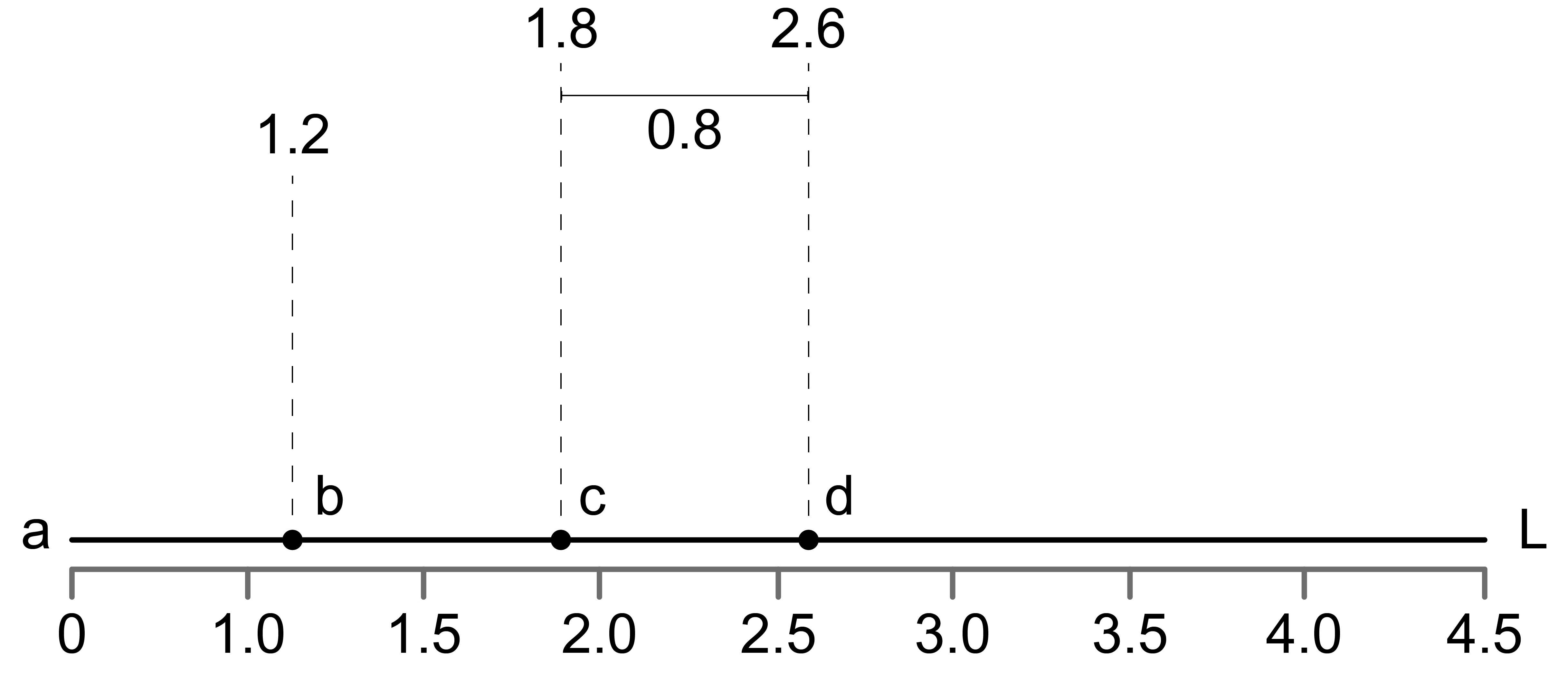
Figure 7.13: Example of using linear referencing to measure distance between points.
In the above figure we can see how linear referencing systems work. Considering one would like to measure distances from node a along a network link L, distance measures can be used to locate, for example, points b, c and d along line L.
7.14 Geocoding
One example of linear referencing is the process of geocoding. Geocoding is the process of converting addresses to geographic coordinates, while reverse geocoding is the process of converting geographic coordinates to addresses (Figure 7.14). In order to achieve this conversion, an address locator uses reference spatial data that are mapped to a geographic or projected coordinate system in order to locate new addresses or coordinates.
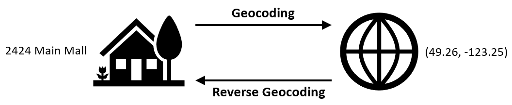
Figure 7.14: Conceptual figure showing the process of geocoding (converting addresses to geographic coordinates) and the process of reverse geocoding (converting geographic coordinates to addresses). Pickell, CC-BY-SA-4.0.
For example, consider that we are looking the 100-block of Main Street in Anytown, Canada. Neighbourhood blocks usually demarcate anywhere between 100 and 1000 unique civic numbers along a street segment. So the 100-block of our conceptual Main Street has addresses in the range of 100-199 (Figure 7.15). It is important to recognize that this is only a segment of Main Street, which presumably extends farther with additional segments for the 200-block, 300-block, and so on. (Remember, with proper planar topology, a single street can be comprised of many segments due to intersections with other streets.)
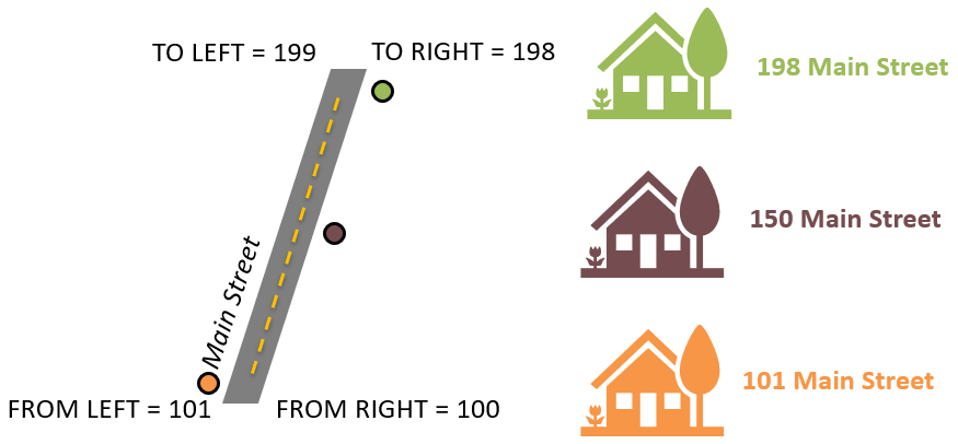
Figure 7.15: The 100-block of Main Street represents all civic addresses in the range of 100-199. Pickell, CC-BY-SA-4.0.
Suppose we have three addresses that we want to locate geographically along this segment: 101 Main Street; 150 Main Street; and 198 Main Street. If this segment of Main Street is mapped in a GIS, then we know the exact geographic coordinates (i.e., latitude and longitude) of the vertices and nodes (ends) of the street segment. Within the attribute table for this segment, we would find four fields: FROM_LEFT; TO_LEFT; FROM_RIGHT; and TO_RIGHT (shown below).
| STREET_NAME | FROM_LEFT | TO_LEFT | FROM_RIGHT | TO_RIGHT |
|---|---|---|---|---|
| Main Street | 101 | 199 | 100 | 199 |
These fields indicate the range of civic numbers and the side of the street segment that a particular range falls on. The typical convention for address assignment within municipalities in Canada is odd-numbered civic numbers are on one side and even-numbered civic numbers are on the other side. In the GIS, these are arbitrarily assigned as \(RIGHT\) or \(LEFT\) sides, but geographically these addresses will occur on the North, East, South, or West “sides” of the street segment.
We can see that the values on the \(LEFT\) side of the street range from 101-199, which are odd-numbered, and the values on the \(RIGHT\) side of the street range from 100-198, which are even-numbered. Since the civic numbers of the street segment are known at the nodes (i.g., 100 and 101 at one end and 198 and 199 at the other end), then we can simply interpolate for any other civic number along the segment and identify the location of our three addresses (Figure 7.15). This interpolation process only places an address on the line segment (i.e., the centre of the street), so the locator must also geographically place the address on the correct side of the street using some offset value (usually in meters) that is usually perpendicular to the street segment.
7.14.1 Geocoding Assumptions and Limitations
One problem might seem obvious here: many cities have a street named Main Street. Therefore, an address locator relies on several pieces of reference spatial data such as maps of road networks, postal codes, cities, provinces or states, and countries. The address locator then works to match the input address against this database of spatial reference data. Thus, geocoding is both imprecise and inaccurate because the address locator relies on several assumptions. The primary assumption is that the input address exists and contains no typos or errors. Data entry by humans is a frequent source of typos and different styles for abbreviations (e.g., “E”, “E.” and “East”). An address locator can still geocode an address that does not exist as long as it is specified correctly, which results in an inaccurate location. If the input address is correct, but incomplete (e.g., “Main Street, Vancouver” is missing civic number, city, and province), then the address locator must match the other provided information against the spatial database (e.g., street name and city), which results in an imprecise location.
In addition to a set of geographic coordinates, one key result from geocoding an address is the match score, which is an indication of how well the address locator was able to match the address against the spatial reference database. The match score usually ranges from 0% (no match) to 100% (perfect match) and the calculation varies depending on how you want to penalize incomplete or incorrect input addresses. Although it is frequently presented as a percentage, the match score is not an indication of accuracy and it really only reflects the confidence by the address locator given the reference spatial database. In other words, a completely inaccurate road network with correct names and civic numbers can conceivably “locate” an address with a 100% match score, but very low accuracy. The final limitation is that you cannot geocode addresses outside of the extent of the spatial data provided to the address locator. For geocoding over large areas, we often rely on geocoding services described in the next section.
7.14.2 Geocoding Services
If you are aiming to geocode addresses in a single city, then it is feasible to manually specify your own address locator using available spatial data such as roads, parcels, neighborhoods, and postal codes. However, for geocoding across large areas, this may not be feasible and you may instead rely on geocoding services that use large databases of reference spatial data. Commercially-available geocoding services are frequently used to provide routing, like Google Maps and Waze. However, these geocoding services do not provide match scores or any other indication of how confident or reliable the matches are.
7.15 Routing
One application of linear referencing is to find routes between nodes is an useful application of spatial networks. This is how mapping tools help us navigate the world by finding the most efficient route to move around the city, for example. (Systems Innovation 2015b).
7.16 Least Cost Paths
Usually multiple paths can be traced along a network to go from one point to another. The notion of cost allow us compare the degree of difficulty needed to cross such paths. With this information, it is possible to rank different routes. In spatial networks, cost usually relate to the necessary distance (either physically or logically) to go from a certain node to another, but they might also represent other aspects such as time, traffic, elevation, current flows, etc. For example, way finding tools that are commonly used to help us to locate and move around in the city usually takes into account multiple costs such as distance, traffic and/or elevation. The least cost path is the easiest way to go from one point of the network to another given some set of factors. The image below shows a simple example of a least cost path between two points considering distance to roads.
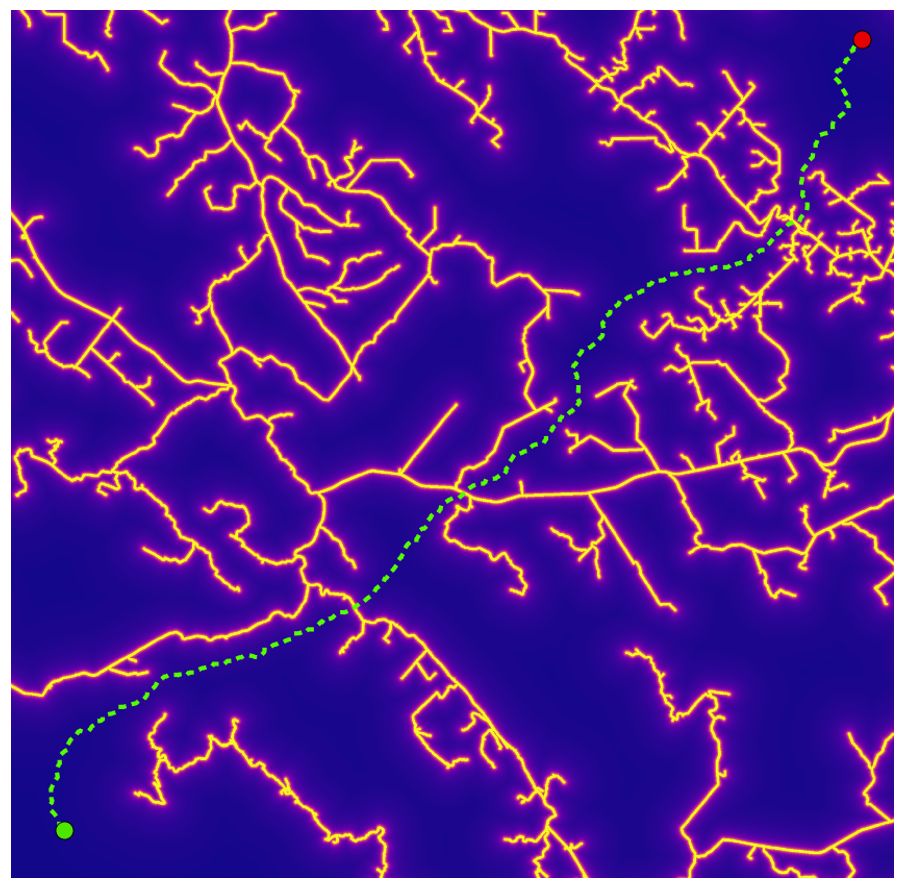
Figure 7.16: Example of a least cost path traced across a cost raster representing distance to road. In this analysis, distance to road is minimized across the entire length of the least cost path. Still, the least cost path must cross several road segments. Pickell, CC-BY-SA-4.0.
Least cost path analysis involves calculating a cost raster. The cost raster represents the total cost of traversing a cell of the raster. In environmental management, we might consider modelling cost factors such as predation risk, terrain, forage quality, preferred habitat, soils, visability, time, and success rate. Each factor can be calculated separately and then combined into a weighted overlay to a final cost raster.
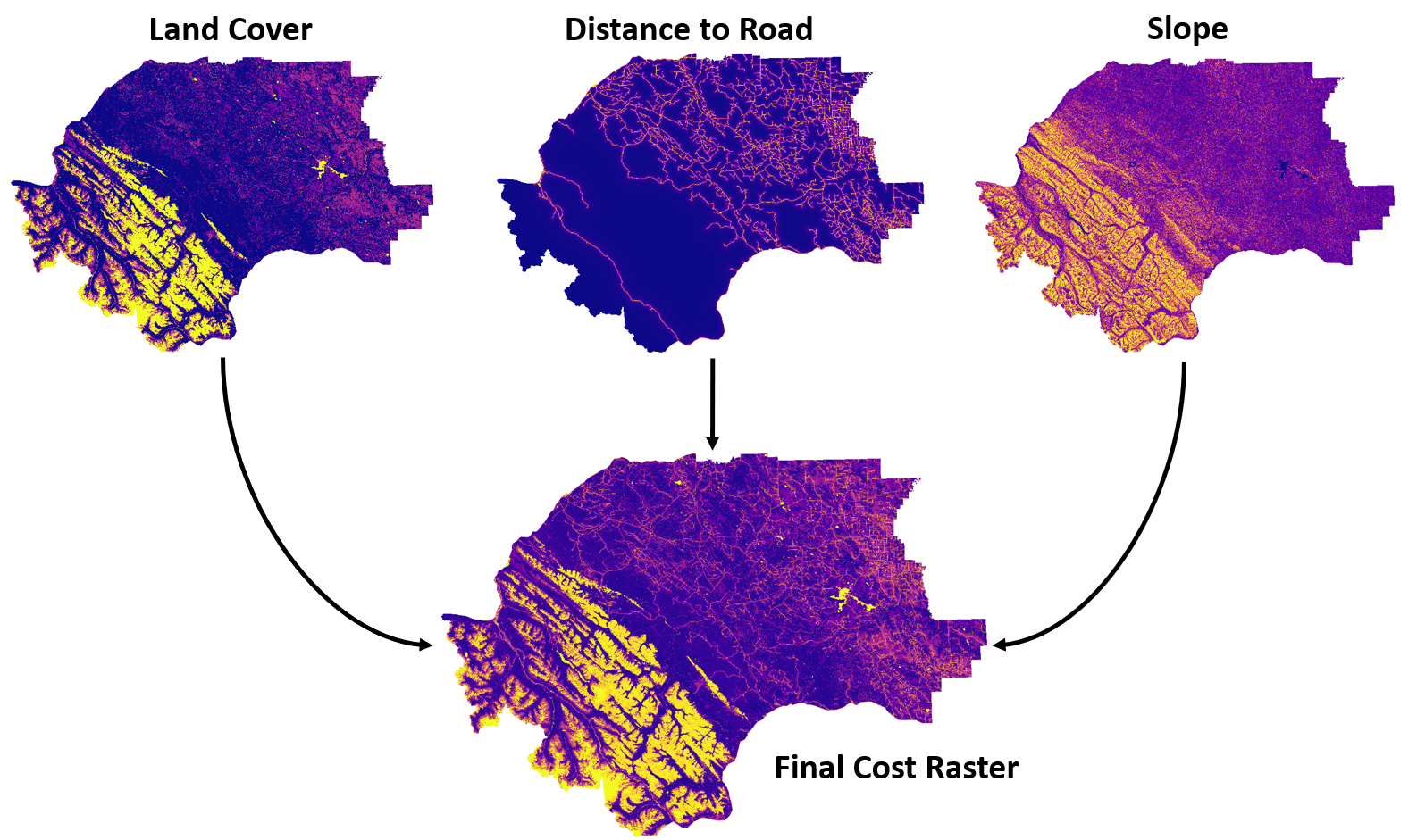
Figure 7.17: Example of calculating a cost raster using three factors in the Yellowhead Grizzly Bear Management Area of Alerta, Canada: land cover, distance to road, and terrain slope. Pickell, CC-BY-SA-4.0.
With the cost raster, we can calculate two other rasters: an accumulative cost raster and a backlink direction raster. The accumulative cost raster represents the total cost to move through a set of cells given a starting point location. In other words, we trace all possible paths leading away from the given point location and add up or accumulate the costs to take that path as illustrated in the image below. The starting point in the least cost path is known as the source location.
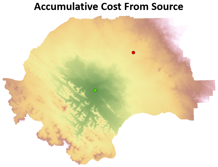
Figure 7.18: Accumulative cost to move from the green source point location. Pickell, CC-BY-SA-4.0.
Given a second point location, we can also calculate an accumulative cost raster for that location as illustrated in the image below. The ending point in the least cost path is known as the target location.
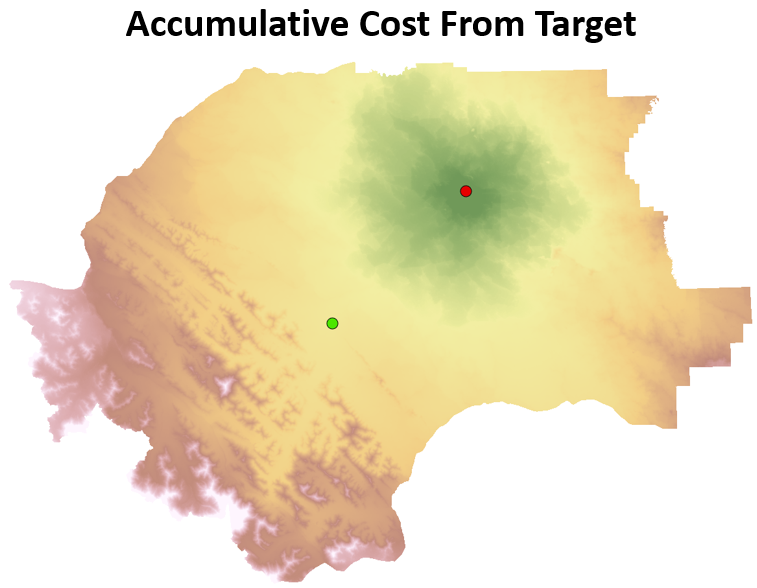
Figure 7.19: Accumulative cost to move from the red target point location. Pickell, CC-BY-SA-4.0.
These two accumulative cost rasters representing the accumulative costs of travelling from the source location and also from the target location can then be added together to produce an accumulative cost raster that represents the accumulative costs to travel between the two locations.
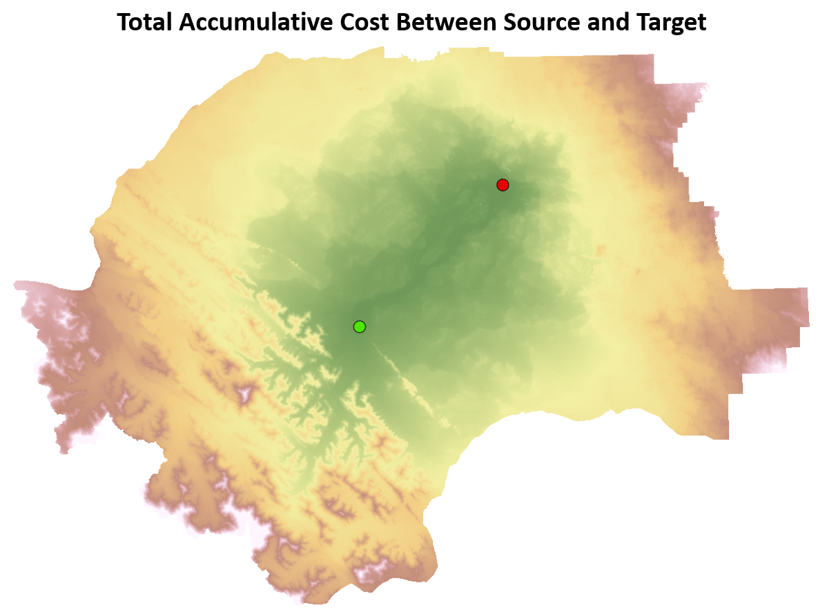
Figure 7.20: Total accumulative cost to move between the green source point location and the red target point location. Pickell, CC-BY-SA-4.0.
Now, in order to solve for the single least cost path, we simply need to trace the path that minimizes the total accumulative cost. This is achieved by encoding a backlink direction for every cell that represents the path to take to return to the source point location. The backlink direction is typically encoded with numbers 0 to 8:
- 0 = Source cell
- 1 = “Move left”
- 2 = “Move upper left”
- 3 = “Move up”
- 4 = “Move upper right”
- 5 = “Move right”
- 6 = “Move lower right”
- 7 = “Move down”
- 8 = “Move lower left”
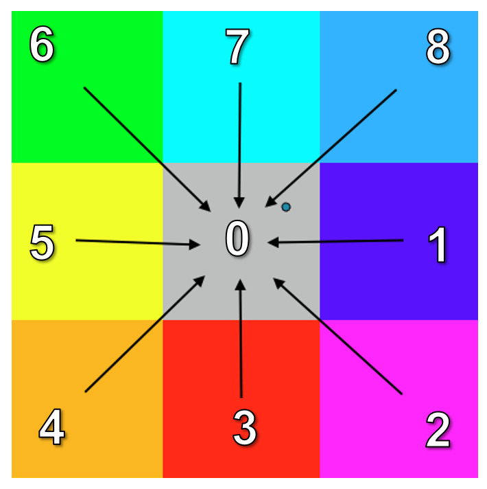
Figure 7.21: The backlink direction is encoded with one of nine numbers that represents the direction for the least cost path to take given any location in the accumulative cost raster. Pickell, CC-BY-SA-4.0.
The backlink encoding is what enables us to trace a path from any target location back to the source location. Think of the backlink raster as a set of instructions that allow us to find our way home in the raster.
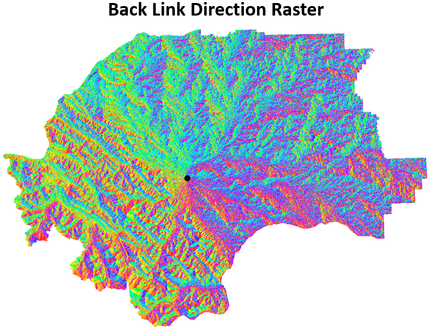
Figure 7.22: Backlink direction raster for the source point location. Pickell, CC-BY-SA-4.0.
With the backlink direction raster, we can now trace the least cost path between the source and target locations. Importantly, because we have an accumulative cost raster that represents the movement costs for all of the possible paths between both locations, we can solve both the least cost path and a least cost corridor. A least cost corridor is an acceptable level or range of costs. For example, we might tolerate any path that has an accumulative cost lower than some cost value. Thresholding the accumulative cost raster in this way allows us to map movement corridors that share the same level of cost. Least cost corridors can be useful for modelling species movement behaviour where many possible paths are tolerable, whereas a least cost path analysis might be more suitable for engineering a forestry road or highway that has specific requirements.
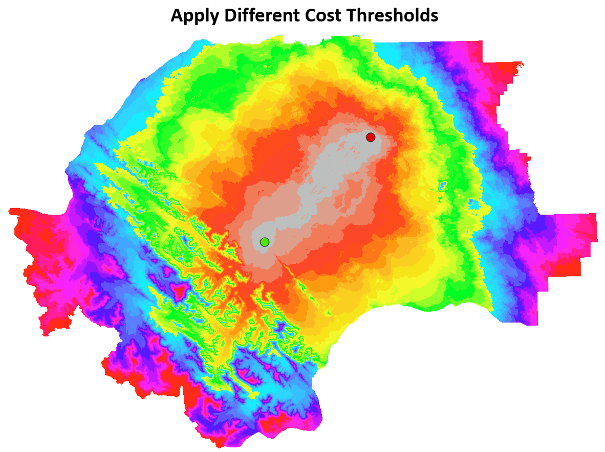
Figure 7.23: Applying thresholds to the accumulative cost raster can reveal least cost corridors rather than a single least cost path. Areas coloured the same represent similar cost tolerance between the green source location and the red target location. Pickell, CC-BY-SA-4.0.
7.17 Reach Analysis
Reach techniques are commonly used to find the incidence of defined elements within a certain radius from a chosen node. All possible routes are modeled. The number of terminal nodes varies according to the network structure. Urban walkability indices usually uses reach techniques to assess the intensity of certain indicators (such as intersection density or non-residential land uses) given a walkable radius (Martino 2020). In the map below we portray the network reach from a given origin point into the Pacific Spirit Regional Park within 400m (red), 800m (yellow), 1200m (green) and 1600m (blue) radii.
Figure 7.24: Reachable segments within multiple distance radii (City of Vancouver n.d.b). Licensed under the Open Government License - Vancouver.
7.18 Network Centrality
Nodes and edges of a graph can also be ranked in terms of how important they are to the overall network. Network centrality measures represent whether elements of a graph are more central or peripheral to the overall system. Such measures can then be interpreted as indicators of importance. Applications are endless. Centrality measures are used for ranking search engine pages (Wikimedia 2021b), for finding persons of interest in social networks (Ajorlou 2018) and for modelling movement in street network (Hillier et al. 1993). There are several centrality measures that serve to the most various purposes. Some of the most commonly used ones are Closeness and Betweenness centrality.
7.19 Closeness Centrality
Closeness centrality measures how close each node is to every other node of the graph in terms of topological distances. It highlights nodes located in easily accessible spaces. For example when analyzing the closeness of street intersections at the University of British Columbia (UBC), intersections in core streets such as the Main Mall, Agronomy Road and Northwest Marine Drive are ranked as highly central whereas more residential and segregated areas such as Acadia Road are ranked with lower closeness centrality.
Figure 7.25: Closeness centrality of the street intersections at UBC (City of Vancouver n.d.b). Licensed under the Open Government License - Vancouver.
Closeness is calculated based on the logical distance from one vertex to all the other vertices in the network. The formula for estimating closeness centrality of a vertex \(i\) is:
\(c_i = \sum\limits_{j} \frac{1}{d_{ij}}\)
where \(d_{ij}\) means the logical distance from \(i\) to \(j\).
7.20 Betweenness Centrality
Betweenness centrality measures how likely a node or an edge is to be passed through when going from every node to every other node of the graph. If we imagine agents travelling from each node to every other node and back, betweenness centrality would be the trail left by those agents. While closeness highlights central spaces, betweenness highlights pathways that lead to those central spaces. Using the same street network at UBC we can calculate the betweenness of segments.
Figure 7.26: Betweenness centrality of street segments at UBC (City of Vancouver n.d.b). Licensed under the Open Government License - Vancouver.
Betweenness is calculated based on the number of shortest paths (in logical distances) from all nodes to all other nodes. According to the documentation of the graph-tool software, betweenness of a vertex \(C_{B}(\upsilon)\) is defined as:
\(C_{B}(\upsilon) = \sum\limits_{s \neq v \neq t \in V} \frac {\sigma_{st}(v)}{\sigma_{st}}\)
where \((v)\) \({\sigma_{st}}\) represents the number of shortest paths from node \(s\) to node \(t\) and \({\sigma_{st}(v)}\) represents the number of those paths that pass through \(v\) (graph-tool n.d.). We can use centrality measures to evaluate how accessible certain spaces are from the point of view of their spatial structure with a broader system.
7.21 Case Study: Central and Peripheral Green Spaces in Vancouver
Are green spaces evenly accessible throughout the whole city? Which parks are topologically closer to the city as a whole? Centrality analysis of the street network can be used to answer these questions.
First we need to find the Closeness measure for the street network of the City of Vancouver. The network information was downloaded from OpenStreetMap. The graph-tool software was used to calculate the centrality measure. With the results of centrality for all street intersections in the city, we can overlay Parks & Green spaces data from the City of Vancouver Open Data portal and get the average closeness of nodes within each green space.
Figure 7.27: Closeness centrality of parks and green spaces at the City of Vancouver (City of Vancouver n.d.b). Licensed under the Open Government License - Vancouver.
Results show parks located in the middle of the city have higher closeness than parks located at the edges. In other words, these parks are located in parts of the city that have easy access to the city’s street network as a whole. As the histogram leans towards the right, we can conclude that there are more parks with higher closeness than parks with lower closeness.
Reflection Questions
- Which types of behaviour can be modelled and understood using network analysis techniques?
- What is the difference between physical and logical distances?
- How can different costs be used for routing along spatial networks?
- How can network centrality measures be interpreted in spatial networks?
- What are some examples of applications of geocoding and reverse geocoding?