Chapter 13 LiDAR Acquisition and Analysis
Written by Francois du Toit and Paul Pickell
Remotely sensed data has traditionally relied on sensors to passively collect reflected energy from the Earth’s surface. As you have read in the preceding chapters, the information that we can derive from these sensors is immense; from landscape level satellite analyses to individual tree vigor assessments. One aspect that is more difficult to characterize however, is what a landscape looks like in three dimensions. LiDAR is changing how we can interpret landscapes and forests by producing it’s own source of energy; this allows us to ask questions not only about the top of the Earth’s surface, but also about the structure of the forest, and what the ground looks like beneath it. In this chapter, we discuss what LiDAR is, as well as how we can use it in multiple different contexts.
- Understand what LiDAR is and how it works
- Understand what we can do with LiDAR data, and what products we can generate
- Understand the basic processing steps required to use LiDAR data for forestry and ecological analysis
Key Terms
Light Detection and Ranging (LiDAR), Laser, Global Navigation Satellite System (GNSS), Inertial Measurement Unit (IMU), Discrete Return, Full Waveform, Surface Models, Area-Based Approach (ABA), Individual Tree Crown Detection (ITD), LiDAR Metrics, Tree Segmentation.
13.1 What is LiDAR?
LiDAR stands for Light Detection And Ranging (sometimes written as lidar, or LIDAR), and is an active remote sensing technology. A laser scanner and time of flight principles are used to collect three dimensional (3D) data. LiDAR systems are made up of three components; a laser-scanning device, an accurate global navigation satellite system (GNSS), and an inertial measurement unit (IMU). The laser-scanning device emits pulses of light and measures the time it takes for energy to be reflected to the device. The GNSS receiver allows the position of the laser to be determined in space, while the IMU records the orientation of the laser (i.e. roll, pitch, and yaw (White et al. 2013)). Figure 13.1 illustrates all of the necessary components of a LiDAR system. When discussing LiDAR in an airborne context (i.e. the unit is being flown), we can call it airborne laser scanning (ALS), and if the unit is in a fixed position on the ground it is called terrestrial laser scanning (TLS).
![Overview of the components of a LiDAR System. As is common for large scale data acquisition, the laser scanning is placed on board an aircarft and scans the Earth below it. The aircraft has on on board GPS/GNSS, as well as an intertial measurement unit (IMU). A GPS base station can be used to post-process data and increase spatial accuracy. 'LiDAR-i lend', [@marek9134_lidar-i_2012], CC-BY-SA-3.0.](images/15-LiDAR-System.png)
Figure 13.1: Overview of the components of a LiDAR System. As is common for large scale data acquisition, the laser scanning is placed on board an aircarft and scans the Earth below it. The aircraft has on on board GPS/GNSS, as well as an intertial measurement unit (IMU). A GPS base station can be used to post-process data and increase spatial accuracy. ‘LiDAR-i lend’, (Marek9134 2012), CC-BY-SA-3.0.
13.2 How Does LiDAR Work?
Typical LiDAR systems use the time of flight method to produce 3D data. A laser ranging instrument produces a short, intense pulse of light from the instrument to a target being measured. Some of this energy is then reflected back to the instrument, where it is recorded (as seen in Figure 13.2). Since the speed of light, and the location of the laser ranging instrument is known, we can calculate the position of the target by timing how long it takes between the the pulse being emitted and received. If we shoot many pulses of light towards a target, we can create a 3D point cloud of our target (see Figure 13.3 for an example of a forest scene). Modern LiDAR systems can emit hundreds of thousands of pulses per second, which means LiDAR point clouds can contain millions of points, and be several gigabytes large.
![Concept of LiDAR. A light signal is emitted by the scanner and reflected off the target. 'Concept of LiDAR', [@cartographer3d_concept_2021], CC-BY-SA-4.0.](images/15-Concept-of-LiDAR.png)
Figure 13.2: Concept of LiDAR. A light signal is emitted by the scanner and reflected off the target. ‘Concept of LiDAR’, (Cartographer3d 2021), CC-BY-SA-4.0.
Since a LiDAR point cloud is a file containing the 3D location of points representing objects on the Earth’s surface, there are several parameters to take note of. It is important to know what the technical specifications of the data collection parameters were (for example, how many points per square meter do we have?), and how the data was collected (what platform was used?). A LiDAR dataset includes several pieces of information for each 3D point. \(X,Y,Z\) location data tells us where each point is (usually to the centimeter scale), and a GPS time stamp is included for each point (\(gpstime\)). Additional information such as \(return\) \(number\), \(scan\) \(angle\), \(classification\), and \(intensity\) are also included with the file, which will be discussed in more detail below (Components of a LiDAR System).
The most common file format for LiDAR files is called the LAS file format (.las). This file format was originally designed for 3D point cloud data, and is a free alternative to proprietary systems or a generic ASCII file interchange system. The main benefits of this file format are that it is relatively quick, can be used by any system, and stores information specific to the nature of LiDAR data without being overly complex (American Society for Photogrammetry & Remote Sensing 2019). More information regarding the file type specifications can be found at their website.
![An example of a typical LiDAR point cloud containing 3.14 million points at approximately 80 points per square meter. The point cloud shows a 200 x 200 meter portion of Pacific Spirit Regional Park in Vancouver, and is part of the [2018 City of Vancouver dataset] (https://opendata.vancouver.ca/explore/dataset/lidar-2018/). Du Toit, CC-BY-SA-4.0.](images/15-las-denoise.png)
Figure 13.3: An example of a typical LiDAR point cloud containing 3.14 million points at approximately 80 points per square meter. The point cloud shows a 200 x 200 meter portion of Pacific Spirit Regional Park in Vancouver, and is part of the [2018 City of Vancouver dataset] (https://opendata.vancouver.ca/explore/dataset/lidar-2018/). Du Toit, CC-BY-SA-4.0.
13.3 LiDAR History and Use
LiDAR for forestry and ecology has been used to monitor vegetation structure, stream properties, and topography among other uses. The earliest versions of LiDAR were known as profiling systems and first investigated in the 1960’s (Nelson 2013). A major limitation of early LiDAR profiling systems were that the system was locked in a near-nadir position (i.e. along-track path), which meant that only transects could be collected, as opposed to a larger swath width as with modern systems (Nelson 2013; Lim et al. 2003). Technological advancements meant that early scanning LiDAR systems became more common in the 1980s, although point densities (measured as points per square meter, points·m-2) were low. Densities of 1-5 points·m-2 limited researchers to area based measurements of forest volume and biomass (Nelson 2013). These limitations were primarily due to the LiDAR sensor, as well as data storage difficulties. Technological improvements such as increased pulse rates and smaller footprints (leading to increased point density), and increased storage capacity have allowed researchers to look as individual trees as well as whole forests (Jakubowski et al. 2013). Previously limited to static LiDAR sensors, ALS point cloud densities of 1000 points·m-2 are now entirely feasible. Figure 13.4 shows two different point clouds densities, and how difficult it would be to delineate individual tree crowns at low point densities.
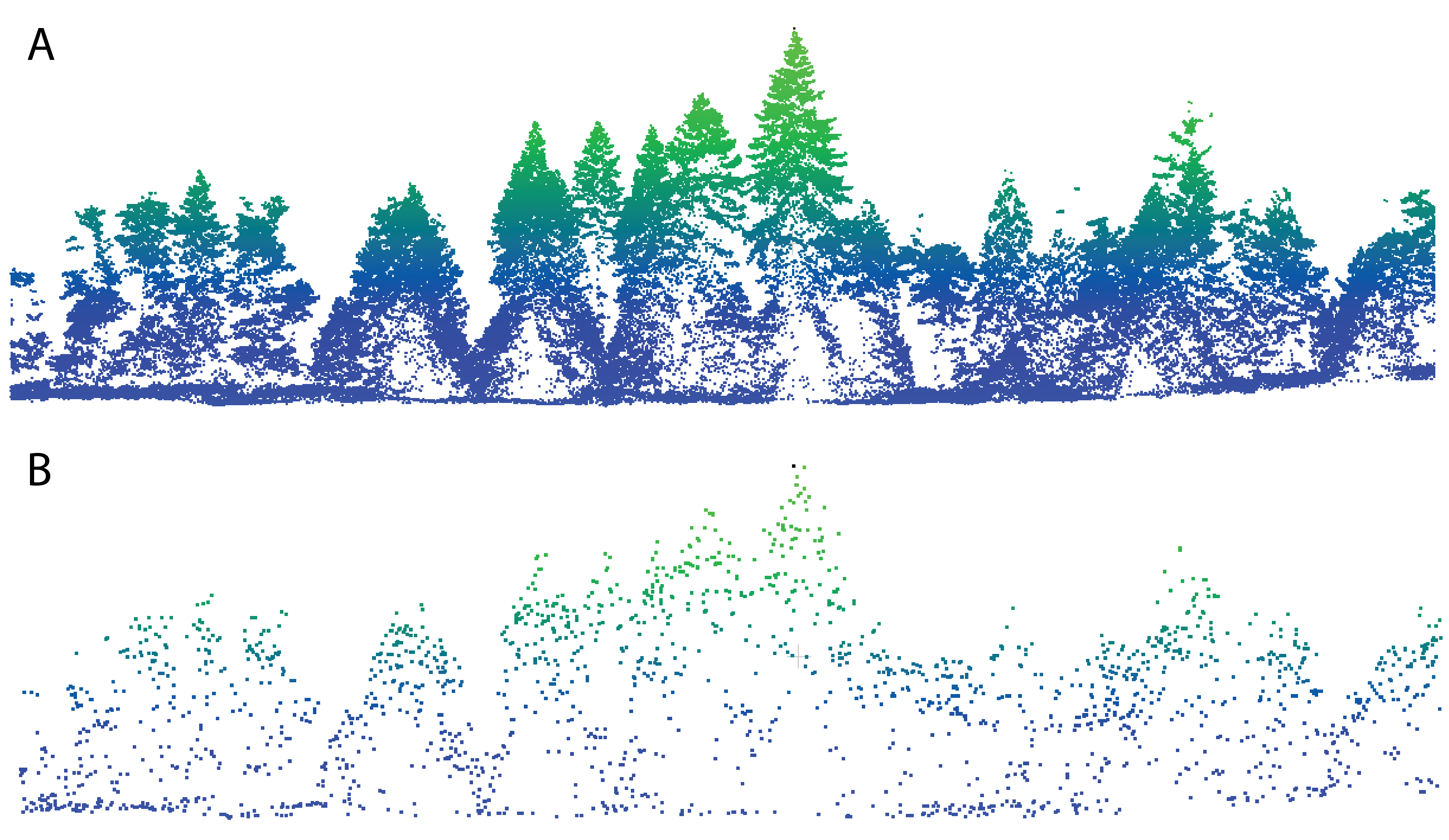
Figure 13.4: A cross section of a high density point cloud (A, 80 points per meter squared), and a lower density point cloud (B, 1 point per meter squared). Du Toit, CC-BY-SA-4.0.
Unlike passive remote sensing technologies, LiDAR has the advantage of being able penetrate forest canopies; this means that we are able to detect the ground, and also characterize both vertical and horizontal vegetation structure. Since the data is extremely accurate, surface models developed using LiDAR are used in many fields where human-made and natural environments need to be mapped. LiDAR derivatives such as surface models are used in hazard assessment (see here: Jaboyedoff et al. (2012)), forestry (read more here: Goodbody et al. (2021)), wet area mapping (here: Eash et al. (2018) and Zurqani et al. (2020)), geologic/geomorphological mapping, and agriculture. In this chapter, we will discuss the use of LiDAR primarily in a forestry context, where raw data and derivatives are used for volume and biomass estimation, as well as individual tree crown analyses.
13.4 Components of a LiDAR System
13.4.1 Lasers
Lasers are a very important component of LiDAR systems. Here we will discuss some basic concepts, as well as the technical parameters that are important when interpreting LiDAR data. LiDAR lasers are typically beams of near-infrared light (800 – 1,550 nm, typically 1,064 nm), and are used because these wavelengths are considered eye safe (White et al. 2013). Green wavelengths are used for bathymetric LiDAR (i.e. water penetrating LiDAR), but are less common, and not typically used on land (UF Geomatics - Fort Lauderdale 2016a). Laser scanners use rotating or oscillating mirrors in order to ‘scan’ a scene in multiple dimensions. When these scanners are placed on a moving platform (e.g. a plane), we can cover large areas. LiDAR sensors scan in a variety of ways: whisk broom, rotation mirror line, and push broom scanners being the most common.
Beam divergence is a property that refers to how wide the light beam becomes when it intercepts an object, and can be used to differentiate LiDAR instruments. Small-footprint LiDAR describes beam diameters intercepting the surface at < 1 m, while large-footprint intercepts the surface at around 5 - 25 m (Lim et al. 2003). Small-footprint LiDAR is primarily what is used in forest inventory and ecology studies, and has high accuracy, as well as the ability to produce high sampling densities. For these studies, beam divergence is typically 0.15 – 2.0 mrad (White et al. 2013). The concept is illustrated in Figure 13.5, and the equation is shown below in (13.1), where \(D\) is the footprint diameter, \(h\) is the flight height (m), and \(\gamma\) is the laser beam divergence (mrad).
\[\begin{equation} D = h \gamma \tag{13.1} \end{equation}\]
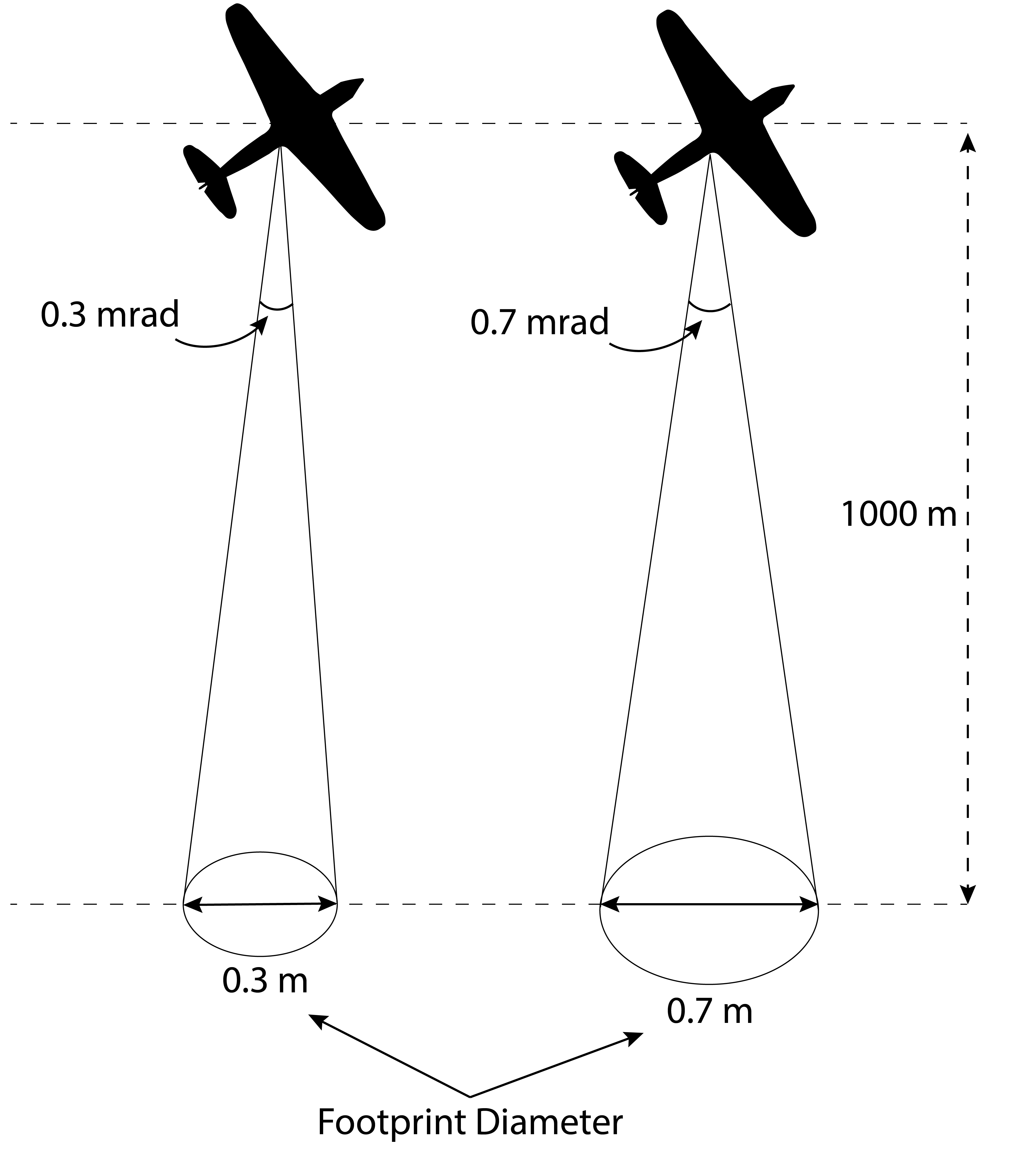
Figure 13.5: Two examples of how beam divergence affects footprint size. Du Toit, CC-BY-SA-4.0.
The amount of energy that is reflected off an object and back to the sensor is known as intensity. Target reflectivity is not directly related to the LiDAR laser itself, but influences whether the return has enough intensity to register with the LiDAR sensor. In addition to surfaces having different properties, the angle of incidence of the laser also affects how much energy the sensor receives. This ‘field of view’ is known as scan angle and can be customized, but lower scan angles are generally preferred (<25°, White et al. (2013)). The concept of scan angle is illustrated in Figure 13.6. Commercial LiDAR units on airplanes typically have stronger lasers than drone mounted or mobile laser scanners, which allows them to fly higher and cover more area.
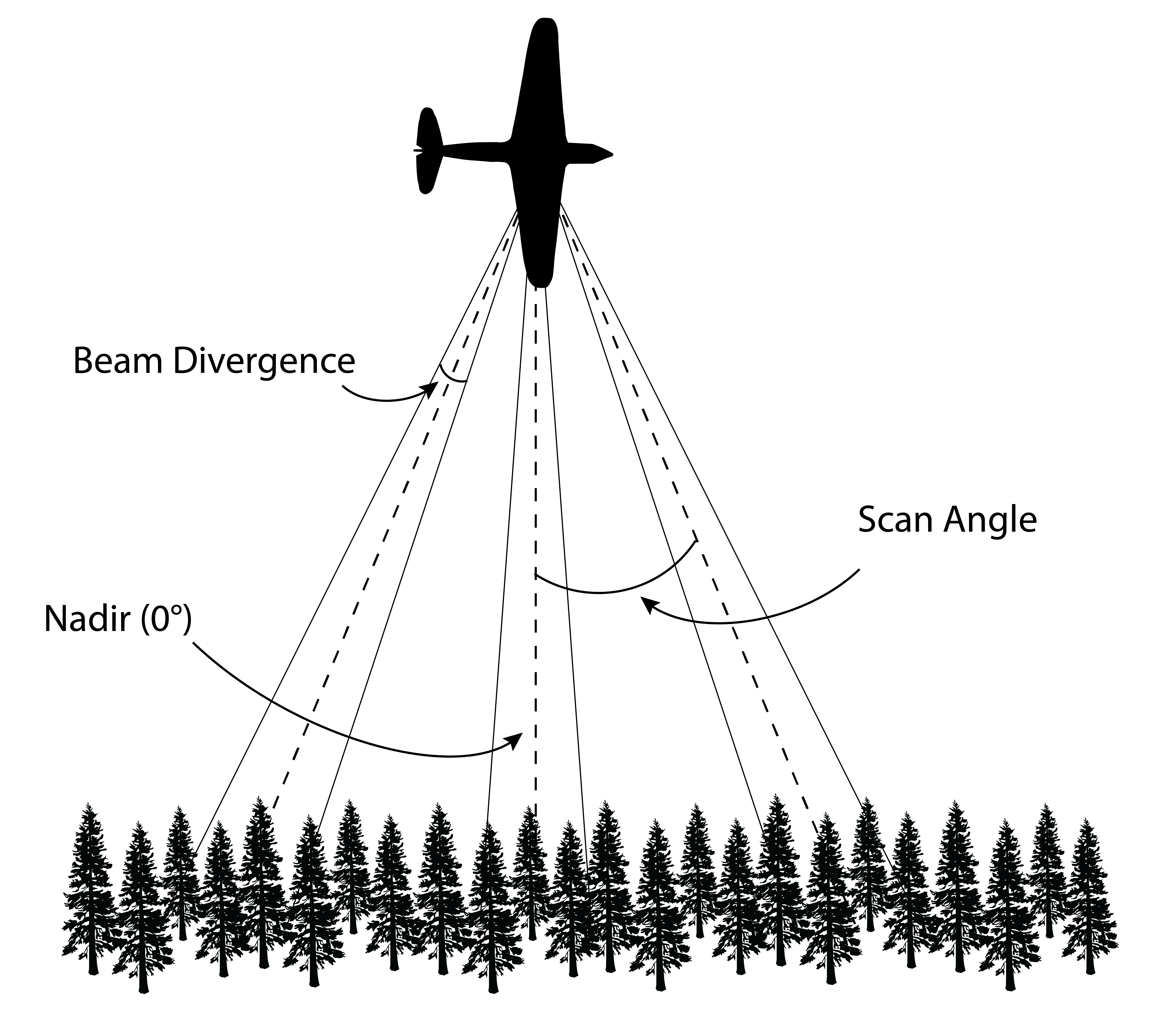
Figure 13.6: Scan angle is the angle from nadir at which the laser is pointing. The scan angle and aircraft flight height together are responsible for swath width. Du Toit, CC-BY-SA-4.0.
All LiDAR sensors emit pulses at a certain rate (pulse rate), which can be given as pulses/second, or hertz (Hz). Pulse rate is highly variable (and often programmable on sensors), and along with scan rate (the number of scan lines per second) and flight speed is responsible for what density a point cloud can be. Pulse rates are commonly 50,000 - 200,000 Hz (White et al. 2013). All of this information means that each LiDAR data acquisition campaign has the potential to be rather unique, and the parameters italicized above need to be taken into account when doing analysis. All of these factors together affect how an individual pulse interacts with the target.
Several technical aspects of lasers are recorded by the instrument (and usually provided as a flight summary or flight specifications by vendors), while some of it can also be found in the las file. We can usually find information that impacts the entire flight in the flight specifications, such as flight height, scan rate, and beam divergence. These aspects shouldn’t change for the entire duration of the flight. In contrast, information located in the las file affects individual points. Here we can find information such as scan angle, return number, and intensity.
![An example of a LiDAR Unit. 'LiDAR machine', [@the_center_for_international_forestry_research_cifor_lidar_2014], CC-BY-NC-ND-2.0.](images/15-LiDAR-Unit.png)
Figure 13.7: An example of a LiDAR Unit. ‘LiDAR machine’, (The Center for International Forestry Research (CIFOR) 2014), CC-BY-NC-ND-2.0.
13.4.2 Global Navigation Satellite Systems
In order for us to use the calculation from Figure 13.2, we need to know the exact position of the scanner in space. For airborne and mobile platforms, we can can do this by using the global navigation satellite system (GNSS), as well as post processing using a local GNSS reference station. This helps us to improve accuracy by not comparing our position to a known local position in order to ensure our location is known as accurately as possible.
![An on board GNSS is required toprovide an accurate location of the LiDAR scanner in space. 'A key component of a lidar system is a GPS', [@neon_education_key_2014], CC-BY-NC-SA-2.0.](images/15-XYZ-coordinates.png)
Figure 13.8: An on board GNSS is required toprovide an accurate location of the LiDAR scanner in space. ‘A key component of a lidar system is a GPS’, (NEON Education 2014), CC-BY-NC-SA-2.0.
13.4.3 Inertial Measurement Unit (IMU)
An inertial measurement unit (IMU) consists of gyroscopes and accelerometers and measures the attitude and acceleration of the aircraft along the X, Y, Z axis. This data is combined with the GNSS data to provide a precise location of the scanner in space. This information becomes very important for airborne platforms where wind conditions can cause the orientation of the scanner to change subtly. We refer to the orientation of the platform in space by using the terms pitch, roll, and yaw, to describe which was the scanner is facing (see 13.1).
13.4.4 Clocks
LiDAR point data needs to be synced with positioning data in order to know exactly where the point is in space. To do this, a very accurate GNSS clock is used to time stamp the laser scanning data (UF Geomatics - Fort Lauderdale 2016b). Accurate clocks are imperative for producing accurate point clouds; one nanosecond (i.e., one billionth of a second) corresponds to a 30 cm travel distance, as seen in Figure 13.11!
13.5 Platform
LiDAR units can be attached to a variety of platforms. Traditionally, LiDAR units for forestry research were mounted on airplanes and helicopters, as units were large and cumbersome, however ground based units such as terrestrial laser scanning (TLS), and mobile laser scanning (MLS) have also been developed. These units tend to have a very high point density, and TLS is often used in modeling tree architecture.
13.5.1 Airplanes and Helicopters
Airplanes and helicopters are still the most common platforms for LiDAR data collection. This is due to their ability to collect large amounts of data in one acquisition. LiDAR units that are designed for airplanes are more powerful than those designed for drones, leading to increased penetration in forests, even though the flight height is significantly increased. Data storage issues can also be mitigated as the platform is not as sensitive to weight restrictions when compared to drones. With increased pulse rates, data acquisitions can also be dense enough to do individual tree crown work. Since helicopters are capable of flying at lower altitudes, slower speeds, and following terrain, they are capable of collecting more dense data, but higher operating costs (White et al. 2013). Typical point densities range from 5 - 200 points·m-2.
13.5.2 Drones
As laser units have decreased in size, we have been able to mount LiDAR units to smaller platforms. Drones (also known as unmanned aerial vehicles (UAV) or remotely piloted aerial systems (RPAS)) are extremely convenient to collect high density point clouds over small areas. They typically fly relatively close to the forest (e.g. 50 m above the trees) and fly a pre-defined flight route so ensure evenly spaced data collection. Typical point densities range from hundreds to thousands of points per meter squared. A major limitation of drones is currently battery life, as acquisition campaigns are limited by how long the drone can fly for (approximately 20 - 30 minutes). This means that collecting large amounts of data is difficult in remote locations.
![Drone mounted LiDAR. This technology is rapidly developing, with many companies working towards creating units capable of acquiring high density datasets over large areas. 'LiDARUSA Snoopy 120 LiDAR', [@mc_clapurhands_lidarusa_2019], CC-BY-SA-4.0.](images/15-LiDAR-on-Drone.png)
Figure 13.9: Drone mounted LiDAR. This technology is rapidly developing, with many companies working towards creating units capable of acquiring high density datasets over large areas. ‘LiDARUSA Snoopy 120 LiDAR’, (Mc Clapurhands 2019), CC-BY-SA-4.0.
13.5.3 Mobile Laser Scanning
Mobile Laser Scanning (MLS) includes people (sometimes called ‘backpack LiDAR’) and moving vehicles. This version of LiDAR has been used by transportation and engineering companies to precisely map things like road or building conditions, and as the units have reduced in size there has been and increase in interest for use in forestry. Current MLS units such as panel 2 in Figure 13.10 can be carried around by the user in a forest easily. The point density for that specific unit is approximately 6,000 points·m-2 while the battery can last for over an hour. Typical point densities are highly dependent on what the MLS is mounted to; and can range from hundreds to thousands of points per square meter.
13.5.4 Terrestrial Laser Scanning
Terrestrial Laser Scanning (TLS) is a static system, meaning that is is placed in one location, takes measurements of a scene, and can then be moved (see panel 1 of Figure 13.10. These units are used by engineers for surveying, and are used by foresters to precisely measure trees. This information can be used to build quantitative structure models (QSM), to precisely estimate tree parameters. Unlike the other platforms mentioned here, TLS is not necessarily a fast data collection technique. Due to occlusion, the TLS instrument needs to be placed in multiple positions around a plot to be able to fully visualize the trees/plot, which means that a one hectare plot can take three to six days to survey (Wilkes et al. 2015)! Typical point densities are in the thousands of points per meter squared.
13.5.5 Satellites
Satellites are a relatively new platform for LiDAR sensors. Two current satellite sensors are highlighted here; ICESat-2 (Ice, Cloud and land Elevation Satellite) and GEDI (Global Ecosystem Dynamics Investigation). Both are examples of large-footprint, profiling LiDAR systems. ICESat-2 was launched in 2018, with the objectives to determine sea-ice thickness and measure vegetation canopy height for large scale biomass estimation (NASA and Neumann 2021). The ICESat-2 LiDAR sensor is composed of 6 beams in 3 pairs, each with a footprint size of 13 m (NASA and Neumann 2021). GEDI is a LiDAR sensor that was installed on the International Space Station in 2018, with 3 lasers producing 10 parallel tracks of observations, and a footprint size of 25 m (NASA and University of Maryland 2021). The GEDI sensor can be seen in panel 4 of Figure 13.10.
![LiDAR Platforms 1: A terrestrial laser scanner (TLS). 'Lidar P1270901.png', [@monniaux_lidar_2007], CC-BY-SA-3.0. 2: A hand-held moblie laser scanner (MLS). Du Toit, CC-BY-SA-4.0. 3: Car mounted MLS. '3D mobile mapping unit', [@oregon_department_of_transportation_3d_2016], CC-BY-2.0'. 4: GEDI, a spaceborne LiDAR sensor. 'A New Hope: GEDI to Yield 3D Forest Carbon Map', [@neon_education_key_2014], CC-BY-2.0.](images/15-LiDAR-Platforms.png)
Figure 13.10: LiDAR Platforms 1: A terrestrial laser scanner (TLS). ‘Lidar P1270901.png’, (Monniaux 2007), CC-BY-SA-3.0. 2: A hand-held moblie laser scanner (MLS). Du Toit, CC-BY-SA-4.0. 3: Car mounted MLS. ‘3D mobile mapping unit’, (Oregon Department of Transportation 2016), CC-BY-2.0’. 4: GEDI, a spaceborne LiDAR sensor. ‘A New Hope: GEDI to Yield 3D Forest Carbon Map’, (NEON Education 2014), CC-BY-2.0.
13.5.6 Discrete Return
Discrete return LiDAR is the most common type of LiDAR. Here, the reflected energy from a pulse is converted into return targets referenced in time and space (White et al. 2013). Discrete return systems can often record multiple returns (often 5 or more), as long as the energy from each return meets the energy threshold to be classified as a return. Returns are classified per pulse, by the arrival sequence in which the return signals are detected by the sensor (UF Geomatics - Fort Lauderdale 2016c). In the case where a laser pulse intercepts a solid object (such as a building), only a single return would occur; in contrast if the laser pulse can penetrate through the object (e.g. the forest), some of the energy will be returned to the instrument where the pulse intercepts stems/branches/leaves (White et al. 2013). Figure 13.11 shows an example of this; a discrete return system would interpret the returned echo as two returns, as there are two peaks in the returned echo corresponding to a canopy and a ground hit. In a forested landscape, first returns often represent the upper canopy, while last returns correspond to the ground or objects near the ground (White et al. 2013).
13.5.7 Full Waveform
Full waveform LiDAR systems record reflected energy from each laser pulse as a continuous signal (White et al. 2013).Traditionally, discrete return systems would only digitally store the discrete returns, without recording the complete analog return (UF Geomatics - Fort Lauderdale 2016c). In contrast, full waveform systems digitize the entire analog signal at high sampling rates (UF Geomatics - Fort Lauderdale 2016c). This can be seen on the right hand side of Figure 13.11. This type of LiDAR creates much larger file sizes which were an issue in the past, but with modern storage capabilities it is becoming a viable alternative to discrete return LiDAR.
![Differents in the response between discrete echo and full waveform LiDAR. 'Airborne Laser Scanning Discrete Echo and Full Waveform signal comparison', [@beck_airborne_2012], CC-BY-SA-3.0.](images/15-LiDAR-Discrete-Full-Waveform.png)
Figure 13.11: Differents in the response between discrete echo and full waveform LiDAR. ‘Airborne Laser Scanning Discrete Echo and Full Waveform signal comparison’, (Anthony Beck 2012), CC-BY-SA-3.0.
Your Turn!
Use our online tool to visualize and explore a discrete return LiDAR point cloud. You can visualize different attributes of the point cloud including elevation, classification, number of returns, return number, and intensity. Why do you think the intensity of returns varies across the vegetation? What do you notice about the pattern of return number relative to the point elevation? What information do you think could be used to classify the returns?
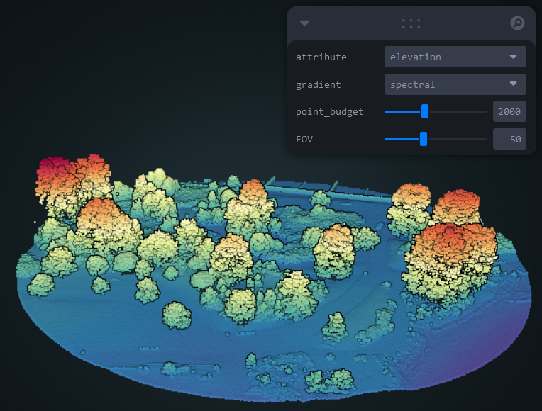
Figure 13.12: Online tool for visualizing and exploring the properties of a small LiDAR point cloud. Data from City of Vancouver and licensed under the Open Government License - Vancouver. Click here to access the interactive tool. Juno Yoon, CC-BY-SA-4.0.
13.6 Emerging Technology
Single Photon LiDAR is an emerging technology that allows wall-to-wall mapping detecting photons reflected off of surfaces more efficiently than traditional LiDAR sensors (Swatantran et al. 2016). While traditional LiDAR systems emit high energy laser beams, single photon systems transmit shorter, lower energy pulses (Swatantran et al. 2016). These systems use a green laser (532 nm), and due to the high efficiency nature of the technology can acquire high density point clouds (12 - 30 points·m-2) up to 30 times faster than traditional systems, and operate at higher altitudes (Swatantran et al. 2016). The system is also capable of penetration semi-porous obscurations such as vegetation, ground fog and thin clouds during daytime and night-time operations (Swatantran et al. 2016).
Multispectral LiDAR units such as the Optech Titan sensor operate three distinct wavelengths of 1,550 nm, 1,064 nm, and 532 nm (Morsy, Shaker, and El-Rabbany 2017). This technology enables 3D spectral information to be captured; for example, NDVI can be calculated for the 3D point cloud. Combining multispectral LiDAR at three wavelengths allows for higher reliability and accuracy compared to single-wavelength LiDAR (Morsy, Shaker, and El-Rabbany 2017), however this technology is not yet widespread.
Specifications for LiDAR data acquisitions are highly variable. It is important to know what type of LiDAR you are using, and to understand the technical specifications of the point cloud before diving into any analysis.
13.7 LiDAR Derivatives and Analysis
LiDAR point clouds require post-processing to be useful. Often, point clouds contain noise that needs to be removed, while the points need to be classified to produce derivatives. Once a point cloud has been cleaned and classified, we can create a variety of products to describe the Earth’s surface, as well as describe vertical characteristics of our point clouds. The most important points to identify in a point cloud are ground and non-ground returns; these points are crucial for deriving surface models, such as: digital elevation models, digital surface models, and canopy height models.
13.8 Bare Earth Elevation
Digital Elevation Models (DEM) are raster products that represent elevation of the Earth’s surface above a reference vertical datum such as sea level (White et al. 2013). Using a classified point cloud, we can isolate the points that are categorized as ground (Classification == 2) and create a raster that represents the ground (see Figure 13.13 below). DEMs are also called digital terrain models (DTMs), although a DTM can include vector features that represent natural features such as river channels, cliffs, ridges, and peaks. DEMs have a variety of uses, from terrain modeling for watersheds, to road design (Jean-Romain Roussel, Goodbody, and Tompalski 2021). In addition to being used on their own, DEMs can be used to normalize point clouds; this is the process of subtracting the ground elevation from a point cloud in order to place the points on a flat plane, so that each point represents the height above the ground, not absolute height. To create a DEM, various interpolation techniques are available, but common algorithms include inverse distance weighting (IDW), kriging, and k-nearest neighbour (KNN).
When creating a DEM from a LiDAR point cloud, there are a few important considerations to make. The first is what resolution the DEM should be created with. The density of the point cloud is what dictates this; if the density of a point cloud is low, there is a lower likelihood of a point representing the ground. This means that a lower resolution DEM should be created. Conversely, high density point clouds can produce higher density DEMs. Additionally, forest/vegetation type is important. Dense, coastal forests in BC are likely to have high canopy cover (and therefore fewer ground points) than the more sparse subalpine forests in the province’s interior.
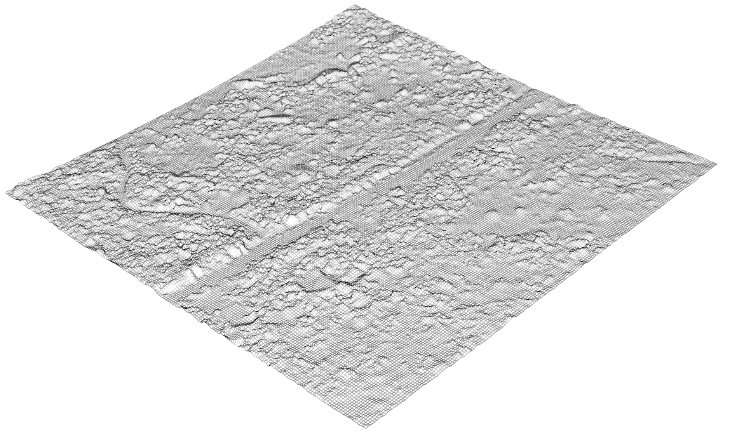
Figure 13.13: A digital elevation model (DEM) produced from LiDAR. Du Toit, CC-BY-SA-4.0.
13.9 Digital Surface Model and Canopy Height Models
Digital surface models (DSMs) represent the height of surface features like trees and buildings above the ground. The ground is defined as the elevation of the terrain above a reference vertical datum. Thus, a DEM is used to reference heights represented in a DSM. In contrast to a DEM, the DSM captures the natural and built features of the environment, and can be thought of as a table cloth placed over a scene. When a point cloud is normalized by subtracting a DEM from a DSM, the derived surface can be called a canopy height model (CHM, Figure 13.14), and represents the height of the canopy above ground level (White et al. 2013). While the elevation values are different, both surfaces can be derived using the same algorithms (Jean-Romain Roussel, Goodbody, and Tompalski 2021).
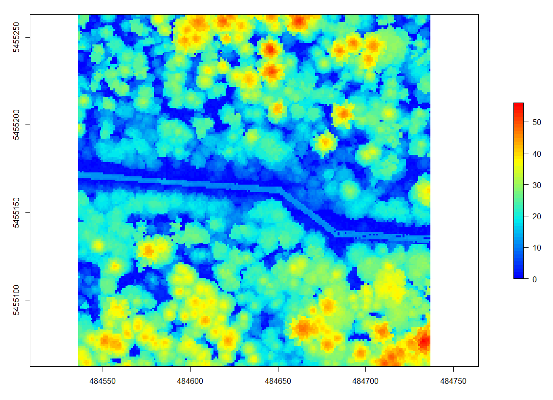
Figure 13.14: A canopy height model (CHM), also known as a digital surface model (DSM) produced from LiDAR. Du Toit, CC-BY-SA-4.0.
13.10 Area Based Approach vs. Individual Tree Crown Approach
LiDAR analysis in forestry uses two broad approaches, an area-based approach (ABA), or an individual tree crown detection approach (ITD). The ITD approach locates individual trees and allows the estimation of individual tree heights and crown area. From this, other metrics such as stem diameter, number of stems, basal area and stem volume can be derived (Hyyppä and Inkinen 1999). In contrast, the main goal of an ABA is to generate wall-to-wall estimates of inventory attributes, such as mean height, dominant height, mean diameter, stem number, basal area, and volume of the stands (Næsset 2002). Since the ABA produces wall-to-wall estimates, the products are usually in a raster format. The ABA approach is what is most often used for forestry inventories, and is an an extensive best practices guide for Canada was produced in 2013 by White et al. (2013). Examples such as Tompalski et al. (2019) show the power that using an ABA can have.
When doing either of these analyses, we typically produce LiDAR metrics. These metrics are descriptive statistics of the point cloud over a unit area; for example Figure 13.15 shows the maximum height of 10 x 10 m cells. How we define that unit is decides what kind of analysis we are able to do, and what kind of inferences are possible (i.e., ABA vs ITD). An ITD approach has a ‘unit’ size of one tree, whereas the ABA typically uses a grid size of 20 x 20 m. Both approaches require ground truthing, and for an ABA approach, plot sizes are typically designed to be of a similar area to the chosen grid size (White et al. 2013).
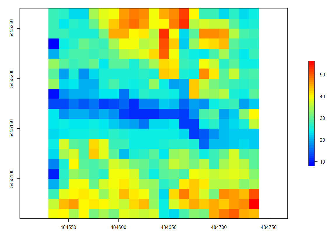
Figure 13.15: Maximum heights of 10 meter cells using an area-based approach. Du Toit, CC-BY-SA-4.0.
13.11 Tree Segmentation
Tree segmentation is required when undertaking an ITD approach. Increased point densities as well as other advancements in LiDAR systems mean that this approach is becoming operationally relevant. Tree segmentation is an attempt to extract individual trees from a point cloud. Since point clouds do not include information regarding what point belongs to which tree, we need to classify the points in a similar way to how we would classify points that represent the ground. Several different algorithms exist in order to detect individual trees and then segments them. Most algorithms follow the logic that tree tops will be near the top of the point cloud, and once the tree top has been identified, a region growing algorithm can be used to ‘grow’ the point cloud downwards.
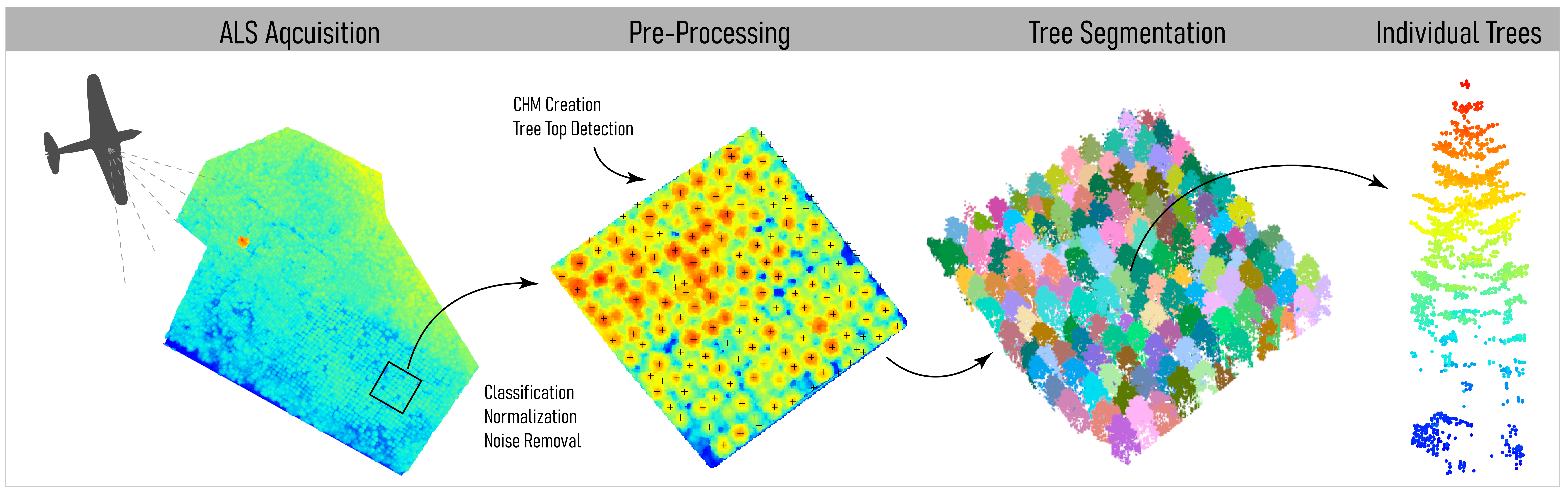
Figure 13.16: A typical LiDAR processing workflow. After acquiring data, pre-processing is necessary to clean and normalize the point cloud. After this a CHM can be created to detect tree tops, before segmentating the point cloud based on these points. Du Toit, CC-BY-SA-4.0.
Once we have segmented a point cloud, we can produce metrics for individual trees. These metrics can be used to help to identify structural traits of trees, which can then be used to identify different tree species, or to characterize different forest types. Ground based LiDAR scanners (MLS and TLS) are also used to very accurately estimate tree, trunk, and branch volumes.
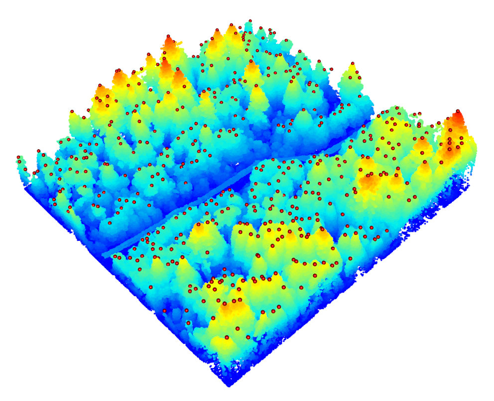
Figure 13.17: Example of tree tops detected using the ‘find trees’ function. Du Toit, CC-BY-SA-4.0.
13.12 Sources of Error
As with other data collection techniques, there are a few sources of error to be aware of. Accuracy of the components are important; if the GNSS is accurate to 1 m, it will cause significant issues compared to a GNSS that is accurate to 2 cm! Additionally, if the IMU has errors, we can have trouble locating ourselves in space, which affects where the laser return is ‘placed’ in 3D space. Typically, we are supplied with estimates of accuracy by the data supplier.
Aside from positional errors, there can also be issues with how we correct for atmospheric conditions, and how it absorbs light. The target surface should also be taken into account, as it can cause multipath errors (where the pulse is reflected off multiple surfaces before returning to the sensor, see Figure 13.18), and occlusion (lasers can not penetrate through solid objects). Finally, areas with highly variable terrain can lead to uncertainty in position, especially when with low density LiDAR.
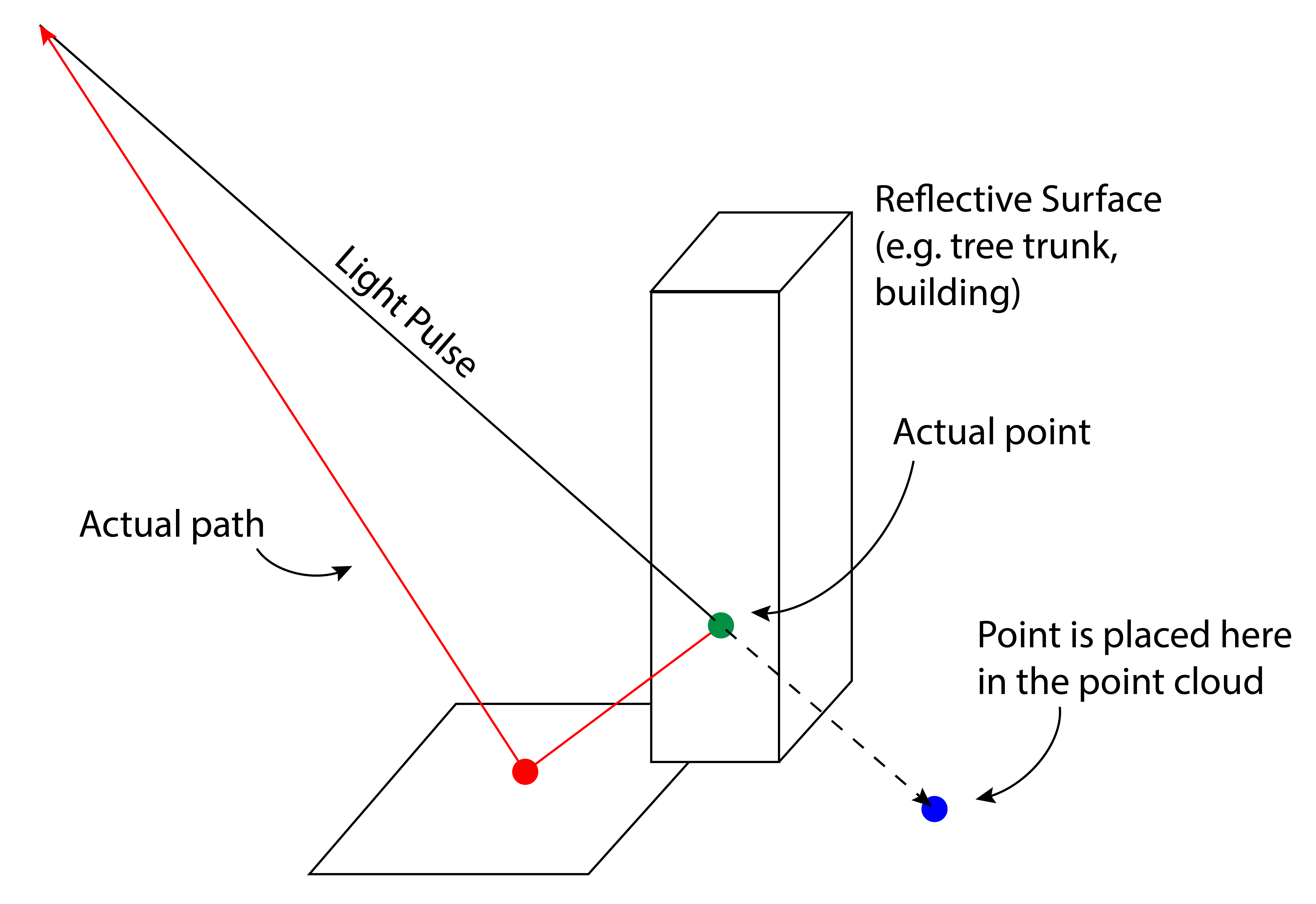
Figure 13.18: Example of multipath errors that can occur. The green dot is where our point is actually located in space, while the blue point shows where the point is placed in the point cloud. The red line shows the path of the reflected pulse. Du Toit, CC-BY-SA-4.0.
13.13 Software and Analysis Tools
As LiDAR acquisition becomes cheaper, more tools are becoming available to do analysis. In this chapter, we use lidR; a free and open source R package that can be used for the entire process of analyzing a point cloud. Several other options exist, such as A Shiny-based Application for Extracting Forest Information from LiDAR data (also in R), the Digital-Forestry-Toolbox which is available for MATLAB, FUSION, a software developed by the USDA Forest Service, and finally QGIS, a free GIS. Paid software is also frequently used in LiDAR processing (examples include ArcGIS Pro, and LAStools), although the cost can be prohibitive. Finally, the open source software CloudCompare can be incredibly useful for both viewing and manually clipping/editing point clouds.
13.14 Case Study: Creating LiDAR Metrics from a Raw Point Cloud
For this case study, we will be using a clipped .las file from the 2018 open LiDAR dataset of the City of Vancouver and UBC Endowment Lands in British Columbia (we randomly selected a 200 x 200 m portion of the ‘4840E_54550N’ tile using CloudCompare), and the lidR package in R (City of Vancouver, n.d.a),(Jean Romain Roussel et al. 2020). The script to process this data is included in the data folder of the GitHub repository, and you can use the lidR book to get a more in depth understanding of the functions we apply below (Jean-Romain Roussel, Goodbody, and Tompalski 2021).
The first step when looking at LiDAR data is to inspect it; we recommend using the free software CloudCompare, or plotting the .las file in the lidR package. Once we have a sense of our data, we can clean and filter the data to remove noise. Our cleaned dataset can then be used to create a DEM; first we need to classify ground points, followed by using an algorithm to rasterize our new ground points to create a surface. This is an essential step that could require quite a bit of tweaking depending on what you want to use the DEM for. It is important to take density into account; a sparse point cloud will not be good for a high resolution DEM! In our case, the DEM is used to normalize the point cloud. Normalization removes the effect of terrain on above ground measurements, allowing comparisons of vegetation heights as you can see in the very uniform point cloud in Figure 13.19.
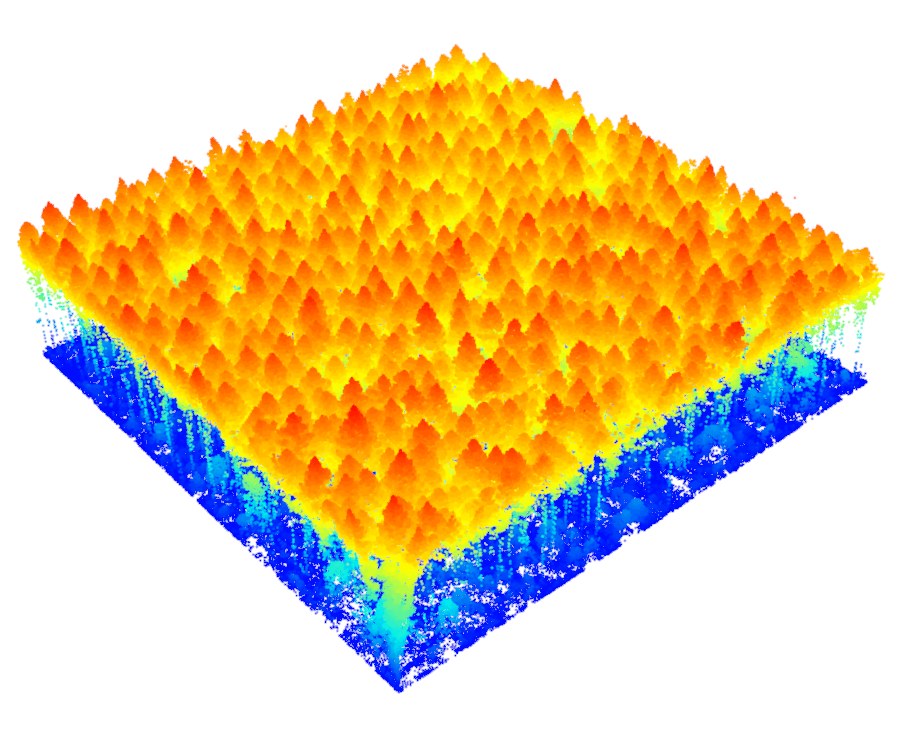
Figure 13.19: A normalized point cloud. Du Toit, CC-BY-SA-4.0.
The normalized point cloud is used to create our CHM. It is at this point that we can analyze the point cloud in a variety of ways. We can use an area-based approach (ABA) to create metrics at the grid level (using our normalized point cloud), or we can derive metrics at the individual tree scale. In order to do this we need to first segment the trees before creating metrics. Segmentation can be tedious, as it requires the user tweak the parameters of their segmentation algorithm. Understanding your forest type, and inspecting the point cloud visually can be very useful when deciding what kind of segmentation routine you want to run. Below we can see an example of a segmented point cloud.
![A segmented point cloud using the algorithm based on [@dalponte_tree-centric_2016]. Du Toit, CC-BY-SA-4.0.](images/15-las-segmented.png)
Figure 13.20: A segmented point cloud using the algorithm based on (Dalponte and Coomes 2016). Du Toit, CC-BY-SA-4.0.
Creating metrics at these two scales are the fundamental way in which we currently think about analyzing forests using LiDAR. Each tells us different things about the forest, so it is important to take scale into account when choosing what kind of analysis you want to do. Below we can see a Leaflet map of some area based metrics created for this point cloud!
Your Turn!
In Figure 13.21 below, explore some of the LiDAR derivatives that we produced in the case study above. We can see how the pattern for maximum height follows the mean height quite closely. In addition, we can see that the 15th percentile of heights (ZQ 15) also broadly follows this pattern. However, we can see that the standard deviation of heights in the tall areas are quite variable, and that very little ground is visible in our tile (as the percentage of points above 2 m is very high almost everywhere).
Figure 13.21: Explore different area-based metrics produced in the case study above. Hover over tile icon (top left) to turn different layers on or off. Du Toit, CC-BY-SA-4.0
13.15 Summary
LiDAR is an active remote sensing technology that requires three components; a laser scanner, a GNSS, and an IMU. The laser scanner emits short, intense pulses of light and measures the time it takes for energy to be reflected back to the device. Time of flight principles are used to produce 3D point clouds, as we know exactly where in space the laser scanner is using the GNSS and IMU. These 3D point clouds can be used to monitor vegetation structure, stream properties, and topography. Point cloud derivatives such surface models can help us analyze different aspects of a forest or landscape. These surfaces can describe the ground (DEM), the top of the Earth’s surface (DSM), or the height of the forest canopy (CHM) when the point cloud is normalized. When using LiDAR in a forestry context, it is important to decide on what resolution we need for our study; we can use an ABA or ITD approach to create LiDAR metrics, which can be used to make different types of inferences about the forest.
Reflection Questions
- What are the three main components of a LiDAR system?
- Why is LiDAR so useful for forestry operations compared to other remote sensing technologies?
- How is a DEM created? What are the main step that are needed?
Practice Questions
- If pulse of light is reflected off a surface 50 m away, what is the travel time of that pulse of light?
- If a plane is flying at 450 m above the ground and the LiDAR sensor has a beam divergence of 0.17 mrad, what is the footprint diameter?
- Explain what is meant by the term ‘discrete return’?
- What is a typical LiDAR wavelength?
Recommended Readings
- A best practices guide for generating forest inventory attributes from airborne laser scanning data using an area-based approach. Information Report FI-X-010 - White et al. (2013)
- Airborne laser scanning for quantifying criteria and indicators of sustainable forest management in Canada - Goodbody et al. (2021)
- Use of LIDAR in landslide investigations: A review - Jaboyedoff et al. (2012)