Chapter 6 Topology and Geocoding
Written by Paul Pickell
Frequently, we need spatial data to behave and relate in specific and predictable ways. Many types of analyses may expect spatial data to be represented and interact in a standard form. In this chapter, we will extend our knowledge of data models using topology, which unlocks many advanced spatial analyses. We will look at a specific example of an analysis that requires topology, geocoding, which will be a convenient segue into network analysis discussed in the following chapter.
- Understand the role of topology in governing data behaviour and data organization
- Recognize some examples and uses of 2D and 3D topologies
- Understand the role of bounding a set of points from triangulation and convex hulls
- Synthesize the process of geocoding
- Practice geocoding addresses and reverse geocoding addresses to other coordinate systems
Key Terms
Vertex, Node, Pseudonode, Dangle, Planar Topology, Non-Planar Topology, Geocoding, Adjacency, Overlap, Connect, Inside, Reverse Geocoding, Singlepart, Multipart, Holes, Delaunay Triangulation, Thiessen Polygons, Voronoi Diagram, Centroid, Convex Hull, Convex Alpha Hull, Multipatch
6.1 Topology
Topology describes the relationships of spatial data. This is a very broad definition that encompasses the wide range of possible arrangements of spatial data in practice. If we drill down into this concept, topology is really what allows us undertake specific types of analysis that requires or expects spatial data to behave in a certain way. If you think about the feature geometries that we have at our disposal, then there are no fewer than nine combinations of how these geometries can interact as illustrated in Figure 6.1 below.
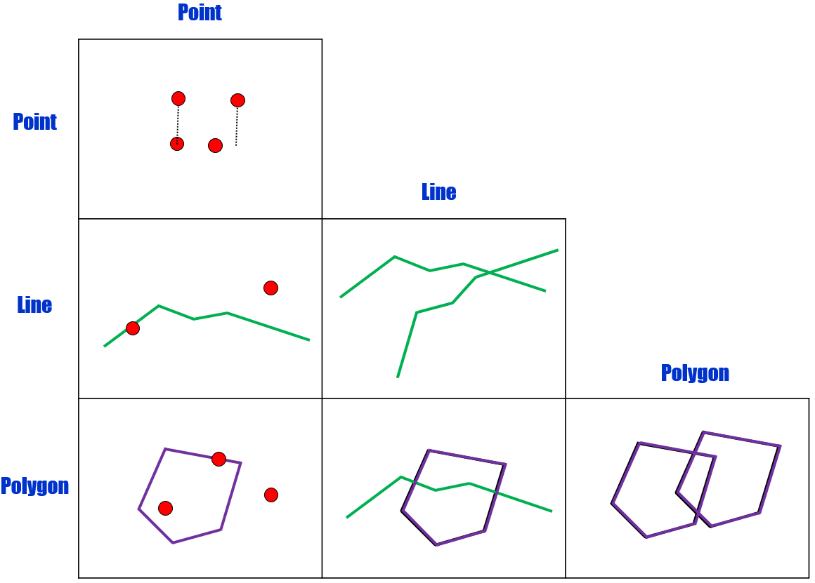
Figure 6.1: Grid showing all the combinations of how point, line and polygon geometries can interact. Pickell, CC-BY-SA-4.0.
It is important to recognize that there may be cases where we “expect” that a given combination of features will conform to a specific interaction. For example, the provinces and territories of Canada are typically represented as polygons that share adjacent boundaries. That is, the adjacent boundaries shared between any two provinces or territories cannot logically overlap as this representation (model) would contravene the legal definitions of the provinces and territories. In another case, a human technician may erroneously digitize a road that crosses another road without indicating that the two roads share an intersection, which could have consequences for how traffic flow can be modeled between the two roads (i.e., intersection with traffic light versus overpass). These are both examples of situations where topology is needed. Topology applies logic to define how features are expected to relate to other features in order to conform to knowledge systems like legal definitions of land and traffic flow. In short, topology ensures data integrity for other types of analysis.
6.2 Planar vs. Non-Planar Topology
In the context of topology, planar refers to the concept that all vertices of feature vector geometry are mapped onto the same plane. So in a planar world-view, all lines and polygons share coincident vertices. For example, if two polygons overlap, then the overlapping area forms a new polygon with a boundary of vertices defined by the union of the two other polygons. Also, if two lines overlap, then the two lines are divided into four new segments and a new vertex is formed at the intersection. In other words, planar topology does not allow polygons or lines to lay “underneath” or “on top” of another line or polygon and feature geometries must always be distinct.
On the other hand, non-planar topology is the concept that vertices of feature vector geometry can be mapped to different planes. It is important to emphasize here that when we are talking about planes that we are not referring to projected coordinate systems. It is generally assumed that any two spatial data layers containing feature geometries are interacting within the same projected coordinate system. Non-planar topology allows for other knowledge systems to be represented in spatial data. The case where a pipeline runs underneath a river or a territory that was traditionally used by several Indigenous peoples (Figure 6.2) are examples of valid non-planar topology.
Figure 6.2: Non-planar topology of 36 indigenous territories overlapping Vancouver Island, British Columbia. Data from Native Land (n.d.), CC0.
6.3 Implementing Planar Topology
Implementing planar topology involves defining specific rules for how features should relate to one another given some analytical context. This process also requires that the spatial data are housed a relational database or data model that supports topology. In other words, topology is enforced only by data models that support topological rules. When a topological rule is violated, the relational database identifies the contravening features and displays them on the map and in the attribute table. Then, it is up to an analyst to decide how the error should be corrected. For example, some errors like intersecting lines can automatically be split at the intersection while overlapping polygons might need to be manually edited to reflect the correct adjacency. Thus, the process of applying topology is first to work within a data model that supports topology, then choose the topological rules that reinforce a particular knowledge system, and finally to inspect and decide how to deal with any contraventions. Since planar topology is only supported by certain data models, and some data models are proprietary to certain software, the exact topological rules that can be implemented in a GIS are mostly dependent on the software that you are using. Instead of examining a specific GIS software package, we will discuss the “fundamental” planar topological relationships that are common across nearly all implementations of topology. (If you want to know more about how topology is implemented within specific data models, skip ahead to the “Data models supporting planar topology” section.)
So far, we have seen that there are six ways to combine feature geometries (points, lines, and polygons). We can extend this understanding to include at least six different ways that they can relate to one another: adjacent; overlap; intersect; connect; cover; and inside. Some of these relationships can be modeled between two different spatial layers (e.g., two point layers) or within a single spatial layer. In the following sections, we will look at different planar topological rules that apply both between and within feature geometries.
6.4 Adjacency and Overlap
There are times when we need to ensure that two polygons are adjacent to one another by sharing a common edge. If two polygons are not adjacent to one another, then a gap, known as a sliver, exists between them or they must overlap. Consider the case where we are mapping land covers. If we have a formal scheme that describes all possible land covers, then we expect that a map of land covers will have perfect adjacency between all polygons so that there are no areas that are not mapped (i.e., slivers) and that no area has multiple, overlapping land covers. Since lines are also 2-dimensional, lines can overlap other lines. Depending on the context, a topological rule may be needed to promote or prevent this relationship. For example, if you are modeling bus routes, then one road might support several different routes.
Figure 6.3: Simplified boundary of Canada (red) and the United States (blue), centred at the Rainy River boundary between Minnesota and Ontario. Without preserving topology, the output results in illogical overlaps in some places and slivers in other places. Pickell, CC-BY-SA-4.0. Data from Natural Resources Canada and licensed under the Open Government Licence - Canada.
Some examples of adjacency and overlap topological rules:
- Polygons within the same layer must not have gaps
- Polygons within the same layer must not overlap
- Polygons must not overlap other polygons
- Lines must not overlap other lines
- Lines must not self-overlap
6.5 Intersect and Connect
As we have seen from Chapter 3, lines are often used to represent phenomena that flow, so intersection and connection are important concepts for these representations. Important to understanding how connection and intersection work in planar topology, we need to understand that lines are comprised of a set of vertices and nodes. A node is simply the terminating vertex in a set of vertices for a line. For example, suppose the line segment \(A\) has a set of vertices, \([[1,0],[1,3],[1,5]]\). Then the nodes for \(A\) are \([1,0]\) and \([1,5]\) (Figure 6.4). Since nodes define the end points of a line segment, they are key to enforcing connection rules. We will look at network analysis in more detail in the next chapter. For now, let us consider two different networks that can help us conceptualize some fundamental line topology using nodes.
![Lines are always comprised of two nodes. Line A shown here has nodes at [1,0] and [1,5]. Pickell, CC-BY-SA-4.0.](geomatics-for-environmental-management-an-open-textbook-for-students-and-practitioners_files/figure-html/7-node-1.png)
Figure 6.4: Lines are always comprised of two nodes. Line A shown here has nodes at [1,0] and [1,5]. Pickell, CC-BY-SA-4.0.
A network of streams and rivers is based on the hydrological knowledge system that explains how water moves over a terrain surface. In both theory and practice, we know that water flows from higher elevations to lower elevations with limited exceptions. Thus, we expect that streams will connect with other streams and continue to flow towards some outlet such as an ocean. Connection refers to the fact that the endpoint node of one stream will fall somewhere on another stream segment. Where two line segments come together, it is possible for one segment \(A\) to “undershoot” the other segment \(B\), resulting in the end node of segment \(A\) appropriately named a dangle (Figure 6.5) and a loss of connection.
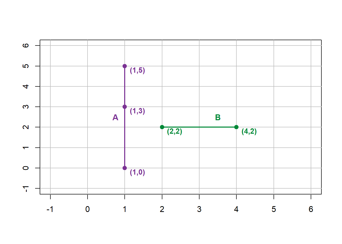
Figure 6.5: A dangle forms when a line (B) does not connect to another line (A). Pickell, CC-BY-SA-4.0.
Dangles are the opposite case to intersections, which occur when two line segments cross each other. With planar topology, intersections must be modeled with a shared node representing the intersection location. For example, suppose line segment \(B\) has a set of vertices, \([[0,1],[2,1],[4,1]]\). If line segments \(A\) (defined above) and \(B\) are mapped together with non-planar topology, then they will intersect at \([1,2]\), which is not a vertex represented in either segment (Figure 6.6).
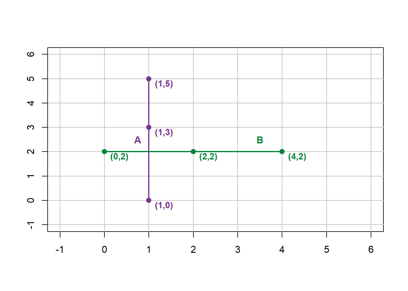
Figure 6.6: Line A mapped with Line B in non-planar topology. Pickell, CC-BY-SA-4.0.
Thus, the intersection of \(A\) and \(B\) with planar topology would yield four new segments: \(C=[[0,2],[1,2]]\), \(D=[[1,2],[1,3],[1,5]]\), \(E=[[1,2],[2,2],[4,2]]\), and \(F=[[1,0],[1,2]]\). Figure 6.7 illustrates how all four of these new segments share the same node \([1,2]\) at the intersection of \(A\) and \(B\).

Figure 6.7: Line A mapped with Line B in planar topology yields segments C, D, E, and F. All segments share (1,2) as a node. Pickell, CC-BY-SA-4.0.
As well, pseudonodes can occur when a node does not actually terminate a line segment at a junction, for example, between two streams or roads. In other words, a pseudonode is a node that is shared by two lines. Figure 6.8 illustrates a pseudonode occurring at \([3,5]\).
![Lines A and B share a pseudonode at [3,5], indicated in red. Pickell, CC-BY-SA-4.0.](geomatics-for-environmental-management-an-open-textbook-for-students-and-practitioners_files/figure-html/7-pseudonode-1.png)
Figure 6.8: Lines A and B share a pseudonode at [3,5], indicated in red. Pickell, CC-BY-SA-4.0.
Some examples of intersection and connection topological rules:
- Lines must not intersect other lines
- Lines must intersect other lines
- Lines must not self-intersect
- Lines within a same layer must not self-intersect
- Lines must not have dangles
6.6 Coincident and Disjoint
Point features can be either coincident or disjoint with other point features. Point features that need to be disjoint may be representing trees, mountain peaks, or any similar type of feature that would be expected to be discrete in geographic space. There are also instances where we might need one set of point features to be coincident with another such as field plots that are centered using a tree or other spatially-discrete feature on the landscape.
Some examples of coincident and disjoint topological rules:
- Points must be disjoint with other points
- Points must by coincident with other points
6.7 Cover
Cover refers to planar topology where a feature lays on or within another feature. For example, dams represented as point features must be covered by a line representing a river (Figure 6.9). Similarly, lines representing rivers must be covered by polygons representing watersheds. As well, property parcel polygons must be covered by the municipal or regional tax authority polygon.
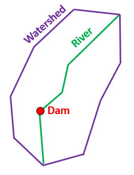
Figure 6.9: Topological relationship between dam (point) covered by a river (line), which is covered by a watershed (polygon). Pickell, CC-BY-SA-4.0.
Some examples of cover topological rules:
- Point must be covered by a line
- Point must be covered by a polygon
- Line must be covered by a polygon
- Polygon must be covered by a polygon
6.7.1 Multipart geometry
Sometimes we need to represent several points, lines or polygons as a collection, which is known as multipart geometry. Multipart geometry allow us to represent several disjoint and non-adjacent geometries as a single feature. In this way, we can assign attribute values to the collection of features rather than each geometry individually. The territorial boundary of Canada is a good example of an instance where a multipart geometry can be useful because all of the contiguous land and non-contiguous land (i.e., islands) can be represented and associated with a single feature in the attribute table. However, if the distinction of features is important, such as identifying the names of islands in the Haida Gwaii archipelago, then a singlepart geometry should be used (Figure 6.10).
Figure 6.10: Singlepart geometry of the Haida Gwaii archipelago off the west coast of British Columbia, Canada. Hover over the islands to see the names. Animated figure can be viewed in the web browser version of the textbook. Polygon data from Statistics Canada (n.d.) and island placenames from Natural Resources Canada (n.d.b). Open Government License - Canada.
Although it is possible to convert from a multipart geometry into singlepart geometry, you need to carefully consider how your features should be represented in the attribute table. For example, if you will be undertaking calculations using area or perimeter of the constituent polygons that comprise a multipart geometry of Canada, then you will return a single value for all of Canada while singlepart geometry would return values for each individual polygon. As well, area calculations can vary between multipart and singlepart geometry. For example, approximately 27% of Canada’s land area (including freshwater), is comprised of more than 52,000 islands, which is a statistic you could only calculate with singlepart geometry. Thus, the choice of representing a feature using singlepart or multipart geometry should be based on how the features will be used in your analysis (i.e., aggregated versus disaggregated).
6.7.2 Holes
When dealing with polygon features, holes may occur, which represent discontinuity of the interior polygon space. Imagine the case of a forested land cover that surrounds a lake. If we consider the forested land cover polygon on its own, then the polygon will have a hole where the lake exists (Figure 6.11).
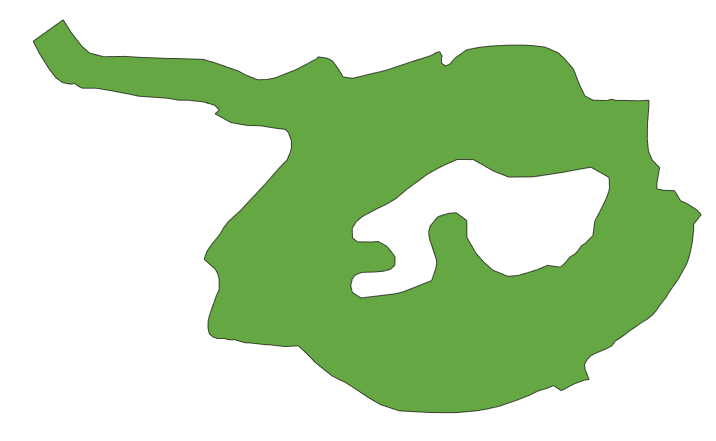
Figure 6.11: Conceptual forest land cover polygon that contains a lake causing a hole. Pickell, CC-BY-SA-4.0.
Topologically, holes in polygons imply that another polygon shares an adjacent boundary where the hole exists, for example, from the union of two layers (see Chapter 6). In our example, the lake would comprise its own polygon that would completely fill the hole.
6.7.3 Delaunay triangulation
Delaunay triangulation is method for forming a triangle mesh over a set of points. The Delaunay triangulation method connects all points in a set such that no point in the set lays within a circumcircle formed by any of the triangles in the mesh (Delaunay 1934). A circumcircle is a circle that passes through all the vertices of a cyclic polygon such as a triangle. In other words, the circumcircles are empty. To illustrate this, consider the four points in Figure 6.12. There are only two circumcircles that can be formed from this set of points that ensures that no point lays within a circumcircle. The triangulation is then simply the lines connecting the three points that fall on any given circumcircle. One important property of the Delaunay triangulation is that the smallest angle in the resulting triangles is maximized from the circumcircle fitting, which minimizes sliver triangles that might from with very shallow angles.
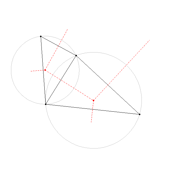
Figure 6.12: Delaunay triangulation of four points. Black lines show the triangulation, grey lines represent the circumcircles connecting the three points of each triangle, red points represent the centres of the circumcircles, and the red dotted lines show that connecting the centres of the circumcircles forms the Voronoi diagram. Pickell, CC-BY-SA-4.0.
Figure 6.13 shows a Delaunay triangulation for a set of 50 points. We can see that sliver triangles mostly occur on the edge of the extent of the points. Delaunay triangulations can be performed both in 2- and 3-dimensional Euclidean space and are therefore important for representing 3D surfaces as well as performing spatial estimation over 2D areas from a set of points.
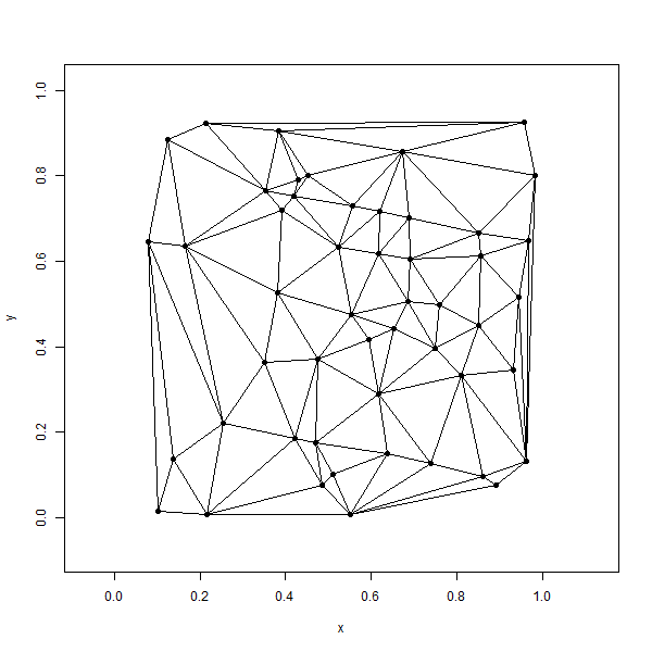
Figure 6.13: Delaunay triangulation of 50 random points. Pickell, CC-BY-SA-4.0.
6.7.4 Thiessen polygons
Thiessen polygons are an implementation of a nearest neighbour algorithm in Euclidean space: given some set of input point features mapped on a plane, partition the plane into polygon areas that represent the nearest locations on the plane to those points. These resulting polygons are also sometimes referred to as proximal polygons, representing the proximal areas given some set of points. When Thiessen polygons are created for geographic data, the resulting diagrams are called Voronoi diagrams and sometimes referred to as Voronoi maps (Figure 6.14). Voronoi maps have many uses such as partitioning geographic space into areas that are nearest to weather stations, airports, or cellular towers. Thiessen polygons can be intersected with other geographic data layers in a GIS using map algebra to efficiently solve proximal questions like, “what is the nearest X?” without having to search or calculate the exact distances of all nearby features, which can be computationally time-consuming (Okabe, Boots, and Sugihara 1994).
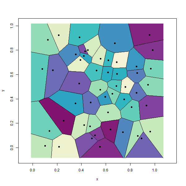
Figure 6.14: Thiessen polygons of 50 random points. Pickell, CC-BY-SA-4.0.
Thiessen polygons are a product of Delaunay triangulation described in the previous section. Figure 6.15 shows the relationship between the points, triangulation, circumcircles, and the Thiessen polygons. Connecting the circumcentres of the circumcircles produces the Voronoi diagram (Figure 6.15).

Figure 6.15: Delaunay triangulation (red lines) overlaid onto the Thiessen polygons. Pickell, CC-BY-SA-4.0.
6.7.5 Centroids
A centroid is a point that represents the geometric centre of a polygon. For convex polygons, the centroid will always lay within the polygon, but for concave polygons, the centroid may lay outside the polygon (Figure 6.16). Circular polygons always have centroids that are equidistant to the boundary of the polygon (Figure 6.17).
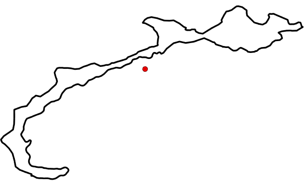
Figure 6.16: Concave polygon with the centroid (red dot) laying outside its boundary. Pickell, CC-BY-SA-4.0.
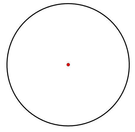
Figure 6.17: Circle polygon with the centroid (red dot) laying equidistant from the boundary of the polygon. Pickell, CC-BY-SA-4.0.
6.7.6 Convex hull
A convex hull is the smallest polygon that contains some set of points. It is sometimes also referred to as a “convex envelope” or “convex closure” because the perimeter of the polygon is formed by connecting the outermost points and closing or enveloping the remaining points. The convex hull is therefore the mathematical implementation of topological closure, where closure refers to the smallest closed set of points that contain the set of points. In practice, the convex hull is a bit like applying a rubber band around the outermost points so that the tension of the rubber band forms straight lines between the pairs of points in the closed set (Figure 6.18). There are several algorithms for computing the convex hull, including Jarvis’ March (Jarvis 1973), Graham’s Scan (Graham 1972), quickhull (Barber, Dobkin, and Huhdanpaa 1996), and CudaHull (Stein, Geva, and El-Sana 2012).
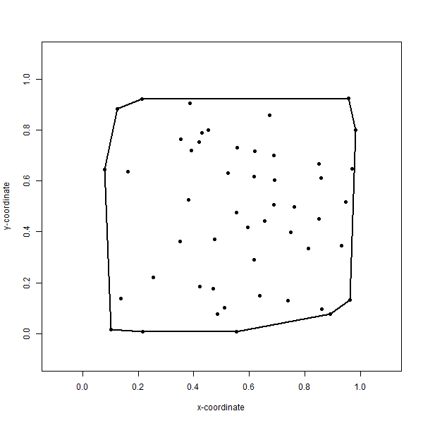
Figure 6.18: Convex hull formed by topological closure of the smallest closed set of points around the entire set of points. Arrangement of the points are the same as in the Thiessen polygons figure above. Pickell, CC-BY-SA-4.0.
6.7.7 Convex alpha hulls and alpha shapes
Convex hulls can be generalized to the concave case, called convex alpha hulls or α-shapes (alpha shapes), by adjusting the maximum radius of the circumcircles through a parameter, alpha \(α\). The objective of a convex alpha hull is to minimize the α-shape formed by circumcircles of radius less than or equal to \(α\). Similar to the Delaunay triangulation, the circumcircles must be open, meaning they contain no other points in the set. Defined in this way, the final α-shape may not result in closure of the full set of points and can result in holes where the distance between points exceeds \(2α\). Surprisingly, α-shapes are prone to not existing at all. For the case of \(α=0\), applying circumcircles of radius 0 results in an empty α-shape and only the input set of points are returned without any boundaries. For \(α=∞\), the α-shape is equivalent to the convex hull because if we use circumcircles with an infinitely large radius, then all points in the set are bound to be enclosed by the resulting α-shape, which like the convex hull must also minimize the bounding area. Figure 6.19 shows an animation of the α-shapes for \(α=1\) to \(α=0\) for our set of 50 points.
Figure 6.19: Concave alpha hull generates an alpha shape around a set of points. Online version of the figure is animated by alpha values from 0 to 1 by increments of 0.05. Animated figure can be viewed in the web browser version of the textbook. Pickell, CC-BY-SA-4.0.
6.8 3D topologies
In this next section, a number of topologies are described that are important for 3D modeling and several examples are given using LiDAR (Light Detection and Ranging), which is the topic of Chapter 15. It is beyond the scope of this chapter to discuss the technology of LiDAR, so the reader is referred to Chapter 15 for a more in-depth discussion of LiDAR.
6.8.1 Multipatch geometries
Similar to multipart geometries, multipatch geometries associate several faces or facets to a single 3D feature such as a building or tree. In order for multipatch geometries to be topologically valid, they must form a closed set of faces, known as a polyhedron. Polyhedrons are comprised of flat faces that connect 3 or more vertices. Figure 6.20 illustrates the 5 Platonic polyhedrons, so-named after Plaot who initially wrote about them. The Platonic polyhedrons are a special type of regular polyhedron because they are the only polyhedrons that are highly symmetrical and have special transitive properties on the edges, faces, and vertices. As well, the Platonic polyhedrons are all examples of the 3-dimensional case of a convex hull (more on that in the next section). Most polyhedrons that we come across in environmental management like trees, lakes, glaciers, and buildings are very irregular and not Platonic.
Figure 6.20: The five Platonic solids are examples of regular, convex polyhedrons and multipatch geometries. From left to right: tetrahedron (4 faces); hexahedron (6 faces); octahedron (8 faces); dodecahedron (12 faces); and icosahedron (20 faces). Animated figure can be viewed in the web browser version of the textbook. Cyp and André (2005), CC-BY-SA-3.0.
6.8.2 3D Convex hull
The 3D convex hull is the smallest convex polyhedron that contains a set of 3D points. The 3D problem is not unlike the 2D problem for finding the 2D convex hull, except instead of using 2D circumcircles we use 3D circumscribed spheres. Otherwise, the overall objective is the same, minimize the 3D polyherdron that encloses the 3D set of points. The 3D convex hull is frequently produced in order to generate a 3D object from a laser scan. Since points are 1-dimensional they have limited use beyond their enumeration within a volume or on a plane or on a line. By contrast, a 3D convex hull produces a polyhedron, which can be used to visualize the object that was initially scanned into a 3D point cloud. The 2D polygon faces that comprise a polyhedron can provide shape and interact with a simulated light source to improve perception of depth, which are qualities that are not provided by 3D points alone.
6.8.3 3D Convex alpha hull
The 3D convex alpha hull is Figure 6.21 below shows a 3D convex alpha hull for a deciduous tree near the Forest Sciences Centre at the University of British Columbia.
Figure 6.21: 3D concave alpha hull for a deciduous tree. The alpha hull was generated using alpha = 0.05. Data collected by Spencer Dakin Kuiper with a GeoSlam terrestrial laser scanner in Vancouver, Canada. Pickell, CC-BY-SA-4.0.
3D concave alpha hull for a deciduous tree. The alpha hull was generated using alpha = 0.05. Data collected by Spencer Dakin Kuiper with a GeoSlam terrestrial laser scanner in Vancouver, Canada. Pickell, CC-BY-SA-4.0.